
Artificial Intelligence Part 1 Search
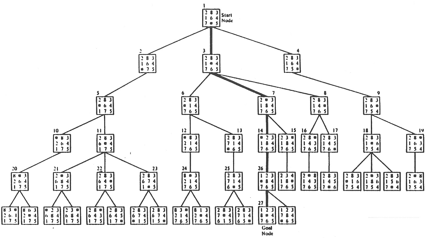 Eight Puzzle Search Tree
Solving the Eight-Puzzle using A-Star and Local Beam Search
Author’s Note: The following is a project I completed for Introduction to Artificial Intelligence at Case Western Reserve University. The complete Python code and documentation can be found on my machine learning GitHub page. One quick comment about my code: as an engineer, I pride myself on getting the job done. That means I often put functionality ahead of clean code. I would appreciate any constructive criticism for optimizing my Python code!
Introduction
The eight puzzle provides an ideal environment for exploring one of the fundamental problems in Artificial Intelligence: searching for the optimal solution path. Although the eight puzzle is a simplified environment, the general techniques of search employed to find the solution can translate into many domains, including laying out components on a computer chip or finding the best route between two cities. Two different search strategies were explored in this project: a-star and local beam search. A-star search was tested with 2 heuristics, while local beam was tested with several values for the beam width.
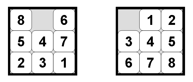 Figure 1: Eight Puzzle in Unsolved and Solved State
Approach
The complete project was coded in Python. The eight_puzzle was implemented as a class with attributes to represent the state of board, a number of utility methods to aid in the solution of the puzzle and visualizing the solution path, and most importantly, the two methods for solving the puzzle. The solution of the eight puzzle is the sequence of blank tile moves that lead from the starting state to the goal state. As the solution is a path, my approach used Python dictionaries to keep track of all nodes considered in each search. Each node includes the current state (the position of all tiles on the board), the parent state, and the action required to get from the parent state to the child state. When the goal state is reached, the algorithm can then transverse backwards through the dictionary starting at the goal state and linking each child state to its parent while recording the series of moves of the blank tile. This solution path can then be displayed and the length of the solution path can be determined. The efficiency of each search can be quantified with an effective branching factor calculated using the length of the solution path and the number of nodes generated during the search.
Code Files
Contains the eight puzzle class with all attributes and methods to represent and solve the puzzle.
Contains code for interacting with the puzzle from the command line or as a series of commands contained in a text file.
Commands for the Eight Puzzle
The following commands can be used to interact with the puzzle from the command line. These commands are implemented as methods of the eight puzzle class.
- -setState [state]
Set the state of the puzzle to the specified argument. The format of the state is “b12 345 678” where each triple represents a row and “b” is the blank tile (the only tile that can be moved).
- -randomizeState [n]
Randomly set the state of the puzzle by taking a random series of n integer actions backward from the goal state. As only half of the initial states of the eight puzzle are solvable, taking a series of steps backward from the goal state ensures that the resulting state will have a solution.
- -printState
Displays the current state of the puzzle in the form “b12 345 678”
- -prettyPrintState
Displays the current state in an aesthetic and understandable format.
- -prettyPrintSolution
Displays the solution as a sequence of moves in an aesthetic and understandable format.
- -move [direction]
Move the blank one place in the specified direction. The move must be one of the following: [“up”, “down”, “left”, “right”] Allowed moves will be determined by the current state of the puzzle.
- -solveAStar [hueristic]
Solve the eight puzzle using the specified heuristic. The choices for the heuristic are ‘h1’ or ‘h2’. ‘h1’ counts the number of misplaced tiles from the goal state while h2 represents the sum of the Manhattan distances of each tile from its correct position in the goal state. After solving the puzzle, the solution path should be printed as a series of actions to move from the starting state to the goal state. The length of the solution path should also be displayed.
- -solveBeam [k]
Solve the eight puzzle using local beam search with the beam width equal to the integer k. In general, a larger value of k is more likely to find a solution becuase the search space is larger, but larger k values will require retaining more nodes in memory. After solving the puzzle, the solution path should be printed as a series of actions to move from the starting state to the goal state. The length of the solution path should also be displayed.
- -maxNodes [n]
The maximum integer n number of nodes to generate during a search. A node is generated when its parent state is expanded. When this limit is exceeded, the code will display an error message. If max nodes is not specified, a default maximum number of 10000 nodes is passed to the method.
- -readCommands [file.txt]
Read and execute a series of commands from a text file. The commands are specified in the same format as the commands for the command line except without the dashes. An example text file is shown below:
setState "3b2 615 748" printState solveBeam 50 maxNodes 2000
Command Implementation
To demonstrate the functionality of the commands, I explain the code that implements the command as well as examples of running the command from the command line. I also show examples of reading commands from a specified text file.
-setState and -printState
setState and printState are both self-explanatory as setState can be used to set the state of the puzzle to any legal configuration and print state can be used to display the state and confirm that the state is as expected. setState checks to make sure that the string is a legal representation of the eight puzzle and then sets the state. printState iterates through the puzzle board and diplays the state in the same format as that used to set the state.
{python}

**def** set_state(self, state_string):
        _# Set the state of the puzzle to state_string in format "b12 345 678"_

        _# Check string for correct length_
        **if** len(state_string) **!**= 11:
            **print**("String Length is not correct!")

        _# Keep track of elements that have been added to board_
        added_elements = []

        _# Enumerate through all the positions in the string_
        **for** row_index, row **in** enumerate(state_string.split(" ")):
            **for** col_index, element **in** enumerate(row):
                _# Check to make sure invalid character not in string_
                **if** element **not** **in** ['b', '1', '2', '3', '4', '5', '6', '7', '8']:
                    **print**("Invalid character in state:", element)
                    **break**
                **else**:
                    **if** element == "b":
                        _# Check to see if blank has been added twice_
                        **if** element **in** added_elements:
                            **print**("The blank was added twice")
                            **break**

                        _# Set the blank tile to a 0 on the puzzle_
                        **else**:
                            self.state[row_index][col_index] = 0
                            added_elements.append("b")
                    **else**:
                        _# Check to see if tile has already been added to board_
                        **if** int(element) **in** added_elements:
                            **print**("Tile {} has been added twice".format(element))
                            **break**

                        **else**:
                            _# Set the correct tile on the board_
                            self.state[row_index][col_index] = int(element)
                            added_elements.append(int(element))

**def** print_state(self):
        _# Display the state of the board in the format "b12 345 678"_
        str_state = []

        _# Iterate through all the tiles_
        **for** row **in** self.state:
            **for** element **in** row:
                **if** element == 0:
                    str_state.append("b")
                **else**:
                    str_state.append(str(element))

        _# Print out the resulting state_
        **print**("".join(str_state[0:3]), "".join(str_state[3:6]), "".join(str_state[6:9]))
The following code block shows an example of setting the state to “325 678 b14” and displaying the result in both string format and prettyPrint format. This command can be run from the command line. The 0 in the pretty printed state is the blank tile.
python play_puzzle.py -setState "325 678 b14" -printState -prettyPrintState

Results:

Current puzzle state:
325 678 b14

Current State
-------------
| 3 | 2 | 5 |
-------------
| 6 | 7 | 8 |
-------------
| 0 | 1 | 4 |
-randomizeState
This method takes a random sequence of “n” allowed moves backwards from the goal state. The resulting state will be solvable. The implementation first sets the state of the puzzle to the goal state, then, for n iterations, the code finds the list of available moves and takes on at random. The state is then set to the result of the move for the next iteration.
{python}

**def** randomize_state(self, n):
        _# Take a random series of moves backwards from the goal state_
        _# Sets the current state of the puzzle to a state thta is guaranteed to be solvable_

current_state = (self.goal_state)

_# Iterate through the number of moves_
        **for** i **in** range(n):
            available_actions, _, _ = self.get_available_actions(current_state)
            random_move = random.choice(available_actions)
            current_state = self.move(current_state, random_move)

_# Set the state of the puzzle to the random state_
        self.state = current_state
The following code block shows an example of randomizing the state by taking 50 random steps from the goal state. The code also displays the state after randomizing in both string format and prettyPrint format.
python play_puzzle.py -randomizeState 50 -printState -prettyPrintState

Results:

Current puzzle state:
154 3b2 678

Current State
-------------
| 1 | 5 | 4 |
-------------
| 3 | 0 | 2 |
-------------
| 6 | 7 | 8 |
-move
This method moves the blank one spot in the specified direction. If the move is not allowed based on the current state of the puzzle, a message is displayed. The move is made as a series of else if statements and the new state is returned as a list.
{python}

**def** move(self, state, action):
        _# Move the blank in the specified direction_
        _# Returns the new state resulting from the move_
        available_actions, blank_row, blank_column = self.get_available_actions(state)

new_state = copy.deepcopy(state)

_# Check to make sure action is allowed given board state_
        **if** action **not** **in** available_actions:
            **print**("Move not allowed\nAllowed moves:", available_actions)
            **return** False

_# Execute the move as a series of if statements_
        **else**:
            **if** action == "down":
                tile_to_move = state[blank_row **+** 1][blank_column]
                new_state[blank_row][blank_column] = tile_to_move
                new_state[blank_row **+** 1][blank_column] = 0
            **elif** action == "up":
                tile_to_move = state[blank_row **-** 1][blank_column]
                new_state[blank_row][blank_column] = tile_to_move
                new_state[blank_row **-** 1][blank_column] = 0
            **elif** action == "right":
                tile_to_move = state[blank_row][blank_column **+** 1]
                new_state[blank_row][blank_column] = tile_to_move
                new_state[blank_row][blank_column **+** 1] = 0
            **elif** action == "left":
                tile_to_move = state[blank_row][blank_column **-** 1]
                new_state[blank_row][blank_column] = tile_to_move
                new_state[blank_row][blank_column **-**1] = 0

**return** new_state
The following two examples first illustrate taking a valid move and then an invalid move. (The puzzle is first set to the goal state for demonstration purposes.)
Valid move: moving “right” from the goal state:
python play_puzzle.py -setState "b12 345 678" -move "right" -printState

Results:

Current puzzle state:
b12 345 678
Invalid move: moving “up” from the goal state:
python play_puzzle.py -setState "b12 345 678" -move "up"

Results:

Move not allowed
Allowed moves: ['right', 'down']
-solveAStar
The main part of the a-star search code is a loop that runs until either a solution is found or the maximum number of nodes is generated. On each iteration, the code finds the available moves from the current state of the puzzle, and then checks to make sure that these moves do not result in a state that has already been expanded or is already on the frontier. If the move satisfies these conditions, the total cost of the move is then evaluated by taking the path cost of the resulting state plus the heuristic of the resulting state (see background on A-Star below). The state that results from the move is then added to the priority queue and at the end of the iteration, the priority queue is sorted by total cost. At the end of each iteration, the best state is chosen from the front of the priority queue and expanded. The node that is expanded will then be added to the expanded_nodes dictionary in order to generate the solution path at the end of the loop. The states that are not expanded on an iteration will be added to the frontier in order to keep track of which nodes have been generated but not expanded. The goal check occurs when a node is expanded rather than when it is generated because it might be possible that the first time the goal state is encountered is not the lowest cost path to the goal. Once a solution is found, the expanded_nodes dictionary is passed to another function that generates and displays the solution path. The total number of nodes generated is the sum of the nodes in the frontier_nodes dictionary and the expanded_nodes dictionary.
Background on A-star search
A-star search is a powerful algorithm for finding an optimal solution path. A-star search chooses the next state based on the total cost of all nodes on the frontier (those that have been generated but not yet expanded). The total cost of a node is defined as
f(state)=g(state)+h(state)
f(state), the total cost of the state, is the sum of g(state), the path cost to get to the state, and h(state), the heuristic function evaluated at the state. In the eight puzzle, the path cost is simply the depth of the state, or the number of moves to get from the start state to the goal state because each move incurs the same cost. The heuristic is either h1, the number of tiles misplaced from their position in the goal state, or h2, the sum of the Manhattan distances of all tiles from their position in the goal state. The heuristic is essentially an estimate of the remaining path distance from the state to the goal.
A-star implements a priority queue, where the frontier nodes in the queue are ordered by total cost with the lowest cost nodes at the front of the queue. Each iteration, the lowest cost node (first in the queue) is expanded and then removed from the queue. My algorithm implements a priority queue, as well as a dictionary to keep track of the expanded nodes and a dictionary to keep track of the nodes on the frontier. The solution path is the sequence of actions from the start state to the goal state, the solution length is the number of actions required, and the number of nodes considered is the number of nodes expanded plus the number of nodes on the frontier.
A-star search is optimal (it finds the shortest solution path) and complete if the heuristic is both admissible and consistent. Admissibility means that the heuristic never overestimates the distance to the goal state. A heuristic is consistent if the estimate to the goal for any node is always less than or equal to the estimate to the goal for any neighboring vertex plus the path cost of reaching that vertex. (This is a general form of the triangle inequality).
Both the h1 and h2 heuristics are admissible and consistent guaranteeing that they will find the optimal solution if it exists. However, the two heuristics are not equally efficient as will be demonstrated in the calculation of the effective branching factors.
{python}

**def** a_star(self, heuristic="h2", max_nodes=10000, print_solution=True):
        _# Performs a-star search_
        _# Prints the list of solution moves and the solution length_

        _# Need a dictionary for the frontier and for the expanded nodes_
        frontier_nodes = {}
        expanded_nodes = {}

        self.starting_state = copy.deepcopy(self.state)
        current_state = copy.deepcopy(self.state)
        _# Node index is used for indexing the dictionaries and to keep_
        _# track of the number of nodes expanded_
        node_index = 0

        _# Set the first element in both dictionaries to the starting state_
        _# This is the only node that will be in both dictionaries_
        expanded_nodes[node_index] = {"state": current_state, "parent": "root",
                    "action": "start",
                    "total_cost": self.calculate_total_cost(0, current_state, heuristic),
                     "depth": 0}

        frontier_nodes[node_index] = {"state": current_state, "parent": "root",
                    "action": "start",
                    "total_cost": self.calculate_total_cost(0, current_state, heuristic),
                     "depth": 0}

        failure = False

        _# all_nodes keeps track of all nodes on the frontier and is the priority queue._
        _# Each element in the list is a tuple consisting of node index and total cost of_
        _#the node. This will be sorted by the total cost and serve as the priority queue._
        all_frontier_nodes = [(0, frontier_nodes[0]["total_cost"])]

        _# Stop when maximum nodes have been considered_
        **while** **not** failure:

            _# Get current depth of state for use in total cost calculation_
            current_depth = 0
            **for** node_num, node **in** expanded_nodes.items():
                **if** node["state"] == current_state:
                    current_depth = node["depth"]

            _# Find available actions corresponding to current state_
            available_actions, _, _ = self.get_available_actions(current_state)

            _# Iterate through possible actions_
            **for** action **in** available_actions:
                repeat = False

                _# If max nodes reached, break out of loop_
                **if** node_index **>**= max_nodes:
                    failure = True
                    **print**("No Solution Found in first {} nodes generated".format(max_nodes))
                    self.num_nodes_generated = max_nodes
                    **break**

                _# Find the new state corresponding to the action and calculate total cost_
                new_state = self.move(current_state, action)
                new_state_parent = copy.deepcopy(current_state)

                _# Check to see if new state has already been expanded_
                **for** expanded_node **in** expanded_nodes.values():
                    **if** expanded_node["state"] == new_state:
                        **if** expanded_node["parent"] == new_state_parent:
                            repeat = True

                _# Check to see if new state and parent is on the frontier_
                _# The same state can be added twice to the frontier if the parent state_
                _# is different_
                **for** frontier_node **in** frontier_nodes.values():
                    **if** frontier_node["state"] == new_state:
                        **if** frontier_node["parent"] == new_state_parent:
                            repeat = True

                _# If new state has already been expanded or is on the frontier,_
                _# continue with next action_
                **if** repeat:
                    **continue**

                **else**:
                    _# Each action represents another node generated_
                    node_index += 1
                    depth = current_depth **+** 1

                    _# Total cost is_
                    _# path length (number of steps from starting state) + heuristic_
                    new_state_cost = self.calculate_total_cost(depth, new_state, heuristic)

                    _# Add the node index and total cost to the all_nodes list_
                    all_frontier_nodes.append((node_index, new_state_cost))

                    _# Add the node to the frontier_
                    frontier_nodes[node_index] = {"state": new_state,
                            "parent": new_state_parent, "action": action,
                            "total_cost": new_state_cost, "depth": current_depth **+** 1}

            _# Sort all the nodes on the frontier by total cost_
            all_frontier_nodes = sorted(all_frontier_nodes, key=**lambda** x: x[1])

            _# If the number of nodes generated does not exceed max nodes,_
            _# find the best node and set the current state to that state_
            **if** **not** failure:
                _# The best node will be at the front of the queue_
                _# After selecting the node for expansion, remove it from the queue_
                best_node = all_frontier_nodes.pop(0)
                best_node_index = best_node[0]
                best_node_state = frontier_nodes[best_node_index]["state"]
                current_state = best_node_state

                _# Move the node from the frontier to the expanded nodes_
                expanded_nodes[best_node_index] = (frontier_nodes.pop(best_node_index))

                _# Check if current state is goal state_
                **if** self.goal_check(best_node_state):
                    _# Create attributes for the expanded nodes and the frontier nodes_
                    self.expanded_nodes = expanded_nodes
                    self.frontier_nodes = frontier_nodes
                    self.num_nodes_generated = node_index **+** 1

                    _# Display the solution path_
                    self.success(expanded_nodes, node_index, print_solution)
                    **break**
The following example shows solving the puzzle from the state “312 475 68b” with a-star using the h1 heuristic and the default number of max nodes (10000). The command can be run from the command line. This puzzle can be solved in four moves and the solution is printed out in a pretty format to see the sequence of moves.
python play_puzzle.py -setState "312 475 68b" -solveAStar h1 -prettyPrintSolution

Results:

Solution found!
Solution Length:  4
Solution Path ['start', 'left', 'up', 'left', 'up', 'goal']
Total nodes generated: 12

Starting State
-------------
| 3 | 1 | 2 |
-------------
| 4 | 7 | 5 |
-------------
| 6 | 8 | 0 |

Depth: 1
-------------
| 3 | 1 | 2 |
-------------
| 4 | 7 | 5 |
-------------
| 6 | 0 | 8 |

Depth: 2
-------------
| 3 | 1 | 2 |
-------------
| 4 | 0 | 5 |
-------------
| 6 | 7 | 8 |

Depth: 3
-------------
| 3 | 1 | 2 |
-------------
| 0 | 4 | 5 |
-------------
| 6 | 7 | 8 |

GOAL!!!!!!!!!
-------------
| 0 | 1 | 2 |
-------------
| 3 | 4 | 5 |
-------------
| 6 | 7 | 8 |
As can be seen, a-star using the h1 heuristic finds the optimal (shortest path cost) solution.
The following example shows what happens if max nodes is specified and the puzzle is not able to find a solution within the maximum number of nodes to consider.
python play_puzzle.py -setState "7b2 853 641" -solveAStar h1 -maxNodes 10

Results:

No Solution Found in first 10 nodes generated
This is an unsolvable puzzle, and as can be seen, no solution is found (try increasing the maximum number of nodes and give your computer some exercise!)
The following example demonstrates solving a randomly generated puzzle taking 10 moves backwards from the goal state. The puzzle is solved with a-star using the h2 hueristic and a maximum of 500 nodes.
python play_puzzle.py -randomizeState 10 -solveAStar h2 -maxNodes 500

Results:

Solution found!
Solution Length:  2
Solution Path ['start', 'left', 'left', 'goal']
Total nodes generated: 5
The algorithm correctly solves the puzzle with both heuristics as demonstrated. The efficiency of the a-star algorithm and a comparison between the two heuristics will be discussed in the effective branching factor section of this report.
-solveBeam
The main part of the local beam search code is a loop that runs until either a solution is found or the maximum number of nodes is generated. Each iteration, all successor states of all current states are generated by finding all available moves. Each successor state is then checked to make sure that it has not already been considered. It if has not, then the algorithm will find the total cost of the state using the evaluation function (see Local Beam Search Background below). The successor states are then added to the priority queue and the queue is sorted by total cost. At the end of the iteration, the k best states (the width of the beam search) are retained from the list of successor states. The k best states then become the current states from which to generate all possible successor states on the next iteration. All nodes are added to a dictionary in order to find the solution path when the loop ends. The goal check occurs when a node is generated because the first time the goal state is encountered represents the end of local beam search. Once the solution is found, the dictionary of all nodes is passed to a function that finds and displays the solution path.
Local Beam Search Background
Local beam search implements a priority queue as in a-star search, but the evaluation function does not take into account the path cost to reach the state. The evaluation function can be defined in any manner as long as it is zero at the goal state. The evaluation function I developed for local beam search is
f(n)=h1(state)+h2(state)
Where f(state) represents the total cost of the state, h1(state) represents the number of misplaced tiles from the goal state of the state, and h2 represents the sum of the Manhattan distances of the tiles in the state from the goal state. This evaluation function was selected because the h1 and h2 heuristics are both consistent and admissible and work well for solving a-star.
A-star considers the path cost to each state when ranking the states whereas local beam only considers the evaluation function of the successor states. In effect, local beam is “blind” to the past and to any future beyond the next step (a-star is also “blind” to the future beyond the next step.) At each iteration, local beam search will calculate the total cost of all successors of all current states and order the successor states by lowest to highest cost. The algorithm will then retain the “k” best states for the next iteration. This limits the amount of states that need to be kept in memory. Local beam search with k=1 is equivalent to hill climbing because the algorithm will just select the successor state with the lowest evaluation function. Local beam search with k=∞ is equal to breadth first search because the algorithm will expand every single state at the current depth before moving deeper in the search tree.
{python}

**def** local_beam(self, k=1, max_nodes = 10000, print_solution=True):
        _# Performs local beam search to solve the eight puzzle_
        _# k is the number of successor states to consider on each iteration_
        _# The evaluation function is h1 + h2, at each iteration, the next set of nodes_
        _# will be the k nodes with the lowest score_

        self.starting_state = copy.deepcopy(self.state)
        starting_state = copy.deepcopy(self.state)
        _# Check to see if the current state is already the goal_
        **if** starting_state == self.goal_state:
            self.success(node_dict={}, num_nodes_generated=0)

        _# Create a reference dictionary of all states generated_
        all_nodes= {}

        _# Index for all nodes dictionary_
        node_index = 0

        all_nodes[node_index] = {"state": starting_state, "parent": "root", "action": "start"}

        _# Score for starting state_
        starting_score = self.calculate_h1_heuristic(starting_state) **+**
                          self.calculate_h2_heuristic(starting_state)

        _# Available nodes is all the possible states that can be accessed_
        _# from the current state stored as an (index, score) tuple_
        available_nodes = [(node_index, starting_score)]

        failure = False

        **while** **not** failure:

            _# Check to see if the number of nodes generated exceeds max nodes_
            **if** node_index **>**= max_nodes:
                failure = True
                **print**("No Solution Found in first {} generated nodes".format(max_nodes))
                **break**

            _# Successor nodes are all the nodes that can be reached from all of the_
            _# available states. At each iteration, this is reset to an empty list_
            successor_nodes = []

            _# Iterate through all the possible nodes that can be visited_
            **for** node **in** available_nodes:

                repeat = False

                _# Find the current state_
                current_state = all_nodes[node[0]]["state"]

                _# Find the actions corresponding to the state_
                available_actions, _, _ = self.get_available_actions(current_state)

                _# Iterate through each action that is allowed_
                **for** action **in** available_actions:
                    _# Find the successor state for each action_
                    successor_state = self.move(current_state, action)

                    _# Check if the state has already been seen_
                    **for** node_num, node **in** all_nodes.items():
                        **if** node["state"] == successor_state:
                            **if** node["parent"] == current_state:
                                repeat = True

                    _# Check if the state is the goal state_
                    _# If the best state is the goal, stop iteration_
                    **if** successor_state == self.goal_state:
                        all_nodes[node_index] = {"state": successor_state,
                                "parent": current_state, "action": action}
                        self.expanded_nodes = all_nodes
                        self.num_nodes_generated = node_index **+** 1
                        self.success(all_nodes, node_index, print_solution)
                        **break**

                    **if** **not** repeat:
                        node_index += 1
                        _# Calculate the score of the state_
                        score = (self.calculate_h1_heuristic(successor_state) **+**
                                    self.calculate_h2_heuristic(successor_state))
                        _# Add the state to the list of of nodes_
                        all_nodes[node_index] = {"state": successor_state,
                                "parent": current_state, "action": action}

                        _# Add the state to the successor_nodes list_
                        successor_nodes.append((node_index, score))
                    **else**:
                        **continue**

            _# The available nodes are now all the successor nodes sorted by score_
            available_nodes = sorted(successor_nodes, key=**lambda** x: x[1])

            _# Choose only the k best successor states_
            **if** k **<** len(available_nodes):
                available_nodes = available_nodes[:k]
The following example demonstrates solving the eight puzzle using local beam search with a beam width of 10 and the maximum number of default nodes (10000). This solution has a true length of 4.
python play_puzzle.py -setState "125 348 67b" -solveBeam 10 -prettyPrintSolution

Results:

Solution found!
Solution Length:  4
Solution Path ['start', 'up', 'up', 'left', 'left', 'goal']
Total nodes generated: 21

Starting State
-------------
| 1 | 2 | 5 |
-------------
| 3 | 4 | 8 |
-------------
| 6 | 7 | 0 |

Depth: 1
-------------
| 1 | 2 | 5 |
-------------
| 3 | 4 | 0 |
-------------
| 6 | 7 | 8 |

Depth: 2
-------------
| 1 | 2 | 0 |
-------------
| 3 | 4 | 5 |
-------------
| 6 | 7 | 8 |

Depth: 3
-------------
| 1 | 0 | 2 |
-------------
| 3 | 4 | 5 |
-------------
| 6 | 7 | 8 |

GOAL!!!!!!!!!
-------------
| 0 | 1 | 2 |
-------------
| 3 | 4 | 5 |
-------------
| 6 | 7 | 8 |
The following example shows randomizing the state with 20 random moves from the goal state, and finding the solution using local beam search with a beam width of 10 and a maximum of 5000 nodes.
python play_puzzle.py -randomizeState 20 -solveBeam 10 -maxNodes 5000

Results:

Solution found!
Solution Length:  8
Solution Path ['start', 'up', 'up', 'right', 'down', 'right', 'up', 'left', 'left', 'goal']
Total nodes generated: 86
Local beam with a beam width of 10 is able to find the solution. However, local beam can get stuck in local optima if the beam width is too narrow.
-readCommands
An additional part of this project was to allow the program to read a sequence of commands from a text file. This was implemented in the play_puzzle.py function using file parsing.
The following example illustrates using a text file to set the state of the puzzle, displaying the initial state of the puzzle, and then solving the puzzle using local beam with a beam width of 50 and 2000 nodes max.
python play_puzzle.py -readCommands "tests\set_state_solve_beam.txt"

Results:

Current puzzle state:
3b2 615 748
Solution found!
Solution Length:  5
Solution Path ['start', 'down', 'down', 'left', 'up', 'up', 'goal']
Total nodes generated: 52
Contents of “set_state_solve_beam.txt”
setState "3b2 615 748" printState solveBeam 50 maxNodes 2000
The following example illustrates using a text file to randomize the state of the puzzle with 16 random steps back from the goal, solving the puzzle using a-star with the h2 heuristic, and pretty printing the solution path in an understandable format.
python  play_puzzle.py -readCommands "tests\randomize_solve_astar.txt"

Results:

Solution found!
Solution Length:  6
Solution Path ['start', 'left', 'down', 'right', 'up', 'left', 'left', 'goal']
Total nodes generated: 19

Starting State
-------------
| 1 | 5 | 0 |
-------------
| 3 | 2 | 4 |
-------------
| 6 | 7 | 8 |

Depth: 1
-------------
| 1 | 0 | 5 |
-------------
| 3 | 2 | 4 |
-------------
| 6 | 7 | 8 |

Depth: 2
-------------
| 1 | 2 | 5 |
-------------
| 3 | 0 | 4 |
-------------
| 6 | 7 | 8 |

Depth: 3
-------------
| 1 | 2 | 5 |
-------------
| 3 | 4 | 0 |
-------------
| 6 | 7 | 8 |

Depth: 4
-------------
| 1 | 2 | 0 |
-------------
| 3 | 4 | 5 |
-------------
| 6 | 7 | 8 |

Depth: 5
-------------
| 1 | 0 | 2 |
-------------
| 3 | 4 | 5 |
-------------
| 6 | 7 | 8 |

GOAL!!!!!!!!!
-------------
| 0 | 1 | 2 |
-------------
| 3 | 4 | 5 |
-------------
| 6 | 7 | 8 |
Contents of “randomize_solve_astar.txt”:
randomizeState 16 solveAStar h2 prettyPrintSolution
The above examples demonstate that the program meets all of the requirements as specified in the project description. The final step of the project is to investigate the efficiency of the two algorithms and the two heuristics. Algorithmic efficiency can best be quantified by the effective branching factor.
Efficiency Calculations
Effective Branching Factor
The branching factor for a specific node is the number of successor states generated by that node. The effective branching factor is an estimate for the number of successor states generated by a typical node. The formula to find the effective branching factor is:
N=b_eff+b_eff²+b_eff³+…+b_eff^d
where N is the total number of nodes generated, b_eff is the effective branching factor, and d is the length of the solution path.
To calculate the effective branching factor, I generated 100 starting states for each solution length from 2 moves to 24 moves (by 2). This was done by taking moves backwards from the goal state with the condition that no state could be repeated twice as shown in the following code.
{python}

_# Generate a list of integers from 2 to 22 by 2_
solution_lengths = list(np.arange(2,24,2))

_# Create a dictionary to store the starting states_
_# The format of the dictionary is number of actions in solution path: starting state_
starting_states = {}

_# Iterate through the wanted solution path lengths_
**for** solution_length **in** solution_lengths:
    **print**(solution_length)
    starting_states[solution_length] = []

    _# Store 100 starting states for each solution length_
    **while** len(starting_states[solution_length]) **<** 100:
        puzzle.set_goal_state()
        states = [puzzle.goal_state]
        **while** len(states) **<** solution_length **+** 1:
            _# Retrieve the possible actions, choose one at random,_
            _# and generate the next state by moving_
            available_actions, _, _ = puzzle.get_available_actions(puzzle.state)
            next_action = random.choice(available_actions)
            new_state = puzzle.move(state = puzzle.state, action = next_action)
            _# If this move is not already in the sequence add it on_
            _# This ensures that the solution length will be equal to the_
            _# specified solution length_
            **if** new_state **not** **in** states:
                states.append(new_state)
                puzzle.state = new_state

        _# Append the starting state to the dictionary_
        starting_states[solution_length].append(states[**-**1])
For each solution path length, there are 100 starting states. To evaluate both algorithms and the two heuristics, I iterated through all of these starting states and solved them using the a-star search with the h1 and h2 heuristics and local beam search using a beam width of 10 and 100. I recorded the number of nodes generated by each algorithm in finding the solution and then took the average across the 100 puzzles.
The average number of nodes generated for each algorithm are shown in the table below:
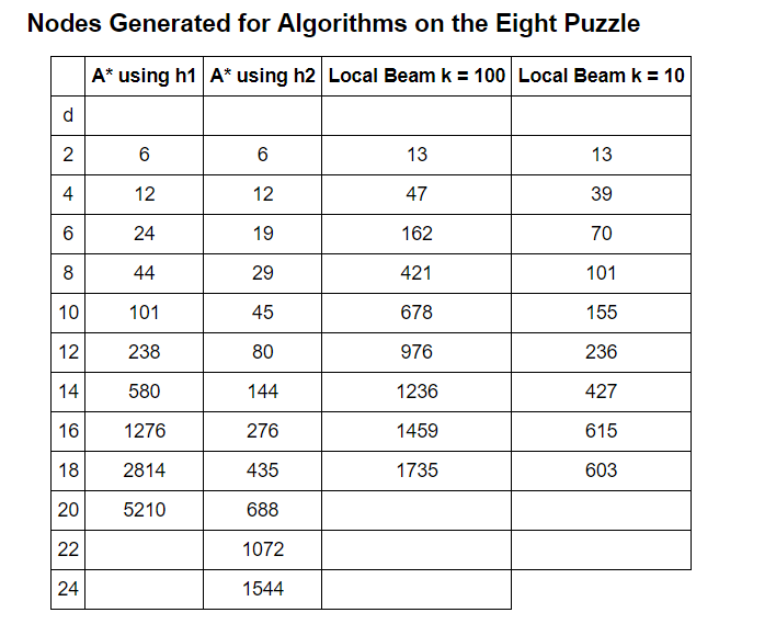 Table 1: Nodes Generated for Each Algorithm Configuration
The effective branching factor can then be calculated by solving the equation described above for b_eff. This equation was solved by moving all terms of the equation to one side and finding the root of the equation graphically. A lower branching factor indicates a more efficient algorithm. As can be seen, the most efficient algorithm tends to be A* using the h2 heuristic with local beam with a beam width of 10 improving as the solution depth increases. If given more time and computing resources, a worthwhile study would be to see if these trends continue as the solution depth increases. The longest solution path to the eight puzzle is 31 moves and if the effective branching factor of local beam continues to decrease, it might be the most efficient algorithm for long solution paths. This makes sense because as the solution depth increases, the benefits of retaining fewer nodes on each iteration will increase. The potential downside of local beam search is that it can become stuck in local optimum and not find the global optimum, or the correct solution path. Local optimum can be avoided using the incredible algorithm known as simulated annealing
The branching factors of the algorithm configurations are summarized in the table below:
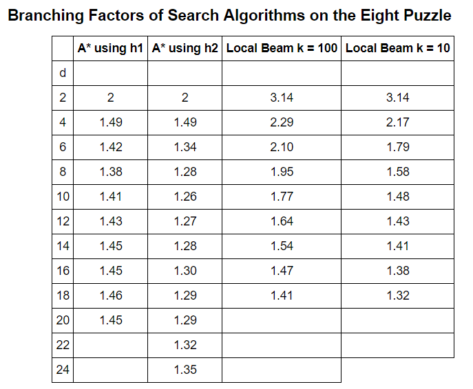 Table 2: Effective Branching Factors of Algorithm Configurations
Visualization of Efficiency
Using the R programming language, I quickly visualized the efficiency of the two algorithms. a_star_h1 refers to the a-star algorithm using the h1 heuristic, a_star_h2 refers to the a-star algorithm using the h2 heuristic, local_beam_10 refers to the local beam algorithm with a beam width of 10, and local_beam_100 refers to the local beam algorithm with a beam width of 100.
{r}

ggplot(generated, aes(d, nodes_generated, color = algorithm)) **+**
geom_jitter(size = 3) **+** geom_line(aes(color = algorithm)) **+**
xlab("Solution Depth") **+** ylab("Nodes Generated") **+**
ggtitle("Nodes Generated vs Solution Depth Broken Out by Algorithm")
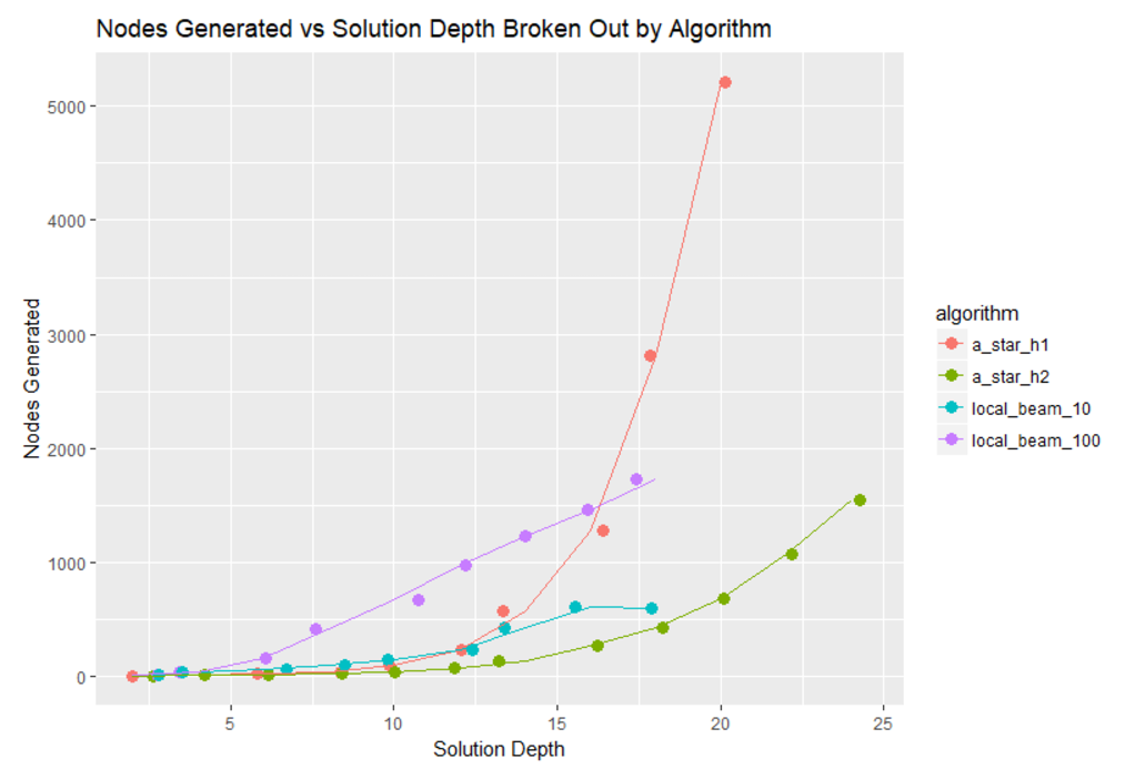 Figure 2: Nodes Generated for Algorithm Configurations
{r}

ggplot(effective, aes(d, effective_branching, color = algorithm)) **+**
geom_jitter(size = 2) **+** geom_line(aes(color = algorithm)) **+**
xlab("Solution Depth") **+** ylab("Effective Braching Factor") **+**
ggtitle("Effective Branching Factor vs Solution Depth Broken Out by Algorithm")
 Figure 3: Effective Branching Factor for Algorithm Configurations
Conclusions
The eight puzzle is a wonderful problem for exploring the basics of search algorithms. This project demonstrated solving the eight puzzle using a-star search with two different heuristics, and using local beam with two beam widths. Further work on the eight puzzle could involve solving the puzzle using a-star search informed by a more sophisticated heuristic such as that developed by Hanson et al in 1992. Another intriguing route for exploration of the eight puzzle would be training a neural network to solve the puzzle using the sequence of actions as a label and the starting state as a feature. Graduate work done by Peterson in 2013 used neural networks to attempt to derive a better heuristic for the eight puzzle. I would like to acknowledge the help provided by the resources linked to in the report as well as the textbook Artificial Intelligence: A Modern Approach by Russell and Norvig. I thoroughly enjoyed developing an eight puzzle solver using search algorithms and am looking forward to greater challenges in artificial intelligence.