How to automatically create machine learning features

Machine learning is increasingly moving from hand-designed models to automatically optimized pipelines using tools such as H20, TPOT, and auto-sklearn. These libraries, along with methods such as random search, aim to simplify the model selection and tuning parts of machine learning by finding the best model for a dataset with little to no manual intervention. However, feature engineering, an arguably more valuable aspect of the machine learning pipeline, remains almost entirely a human labor.

Feature engineering, also known as feature creation, is the process of constructing new features from existing data to train a machine learning model. This step can be more important than the actual model used because a machine learning algorithm only learns from the data we give it, and creating features that are relevant to a task is absolutely crucial (see the excellent paper “A Few Useful Things to Know about Machine Learning”).

Typically, feature engineering is a drawn-out manual process, relying on domain knowledge, intuition, and data manipulation. This process can be extremely tedious and the final features will be limited both by human subjectivity and time. Automated feature engineering aims to help the data scientist by automatically creating many candidate features out of a dataset from which the best can be selected and used for training.

In this article, we will walk through an example of using automated feature engineering with the featuretools Python library. We will use an example dataset to show the basics (stay tuned for future posts using real-world data). The complete code for this article is available on GitHub.

Feature Engineering Basics

Feature engineering means building additional features out of existing data which is often spread across multiple related tables. Feature engineering requires extracting the relevant information from the data and getting it into a single table which can then be used to train a machine learning model.

The process of constructing features is very time-consuming because each new feature usually requires several steps to build, especially when using information from more than one table. We can group the operations of feature creation into two categories: transformations and aggregations. Let’s look at a few examples to see these concepts in action.

A transformation acts on a single table (thinking in terms of Python, a table is just a Pandas DataFrame ) by creating new features out of one or more of the existing columns. As an example, if we have the table of clients below

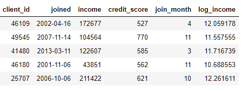
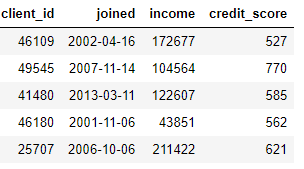we can create features by finding the month of the joined column or taking the natural log of the income column. These are both transformations because they use information from only one table.

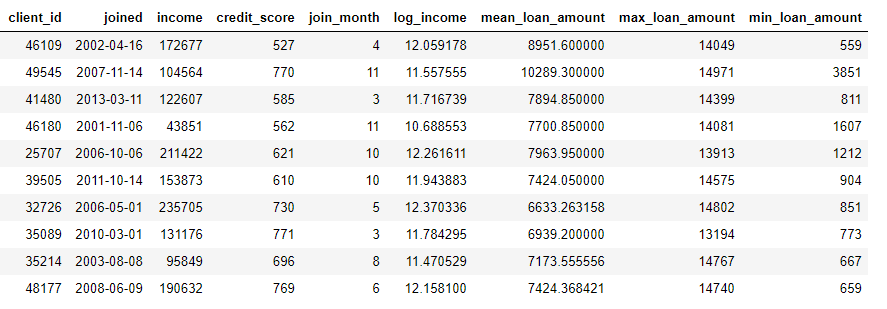
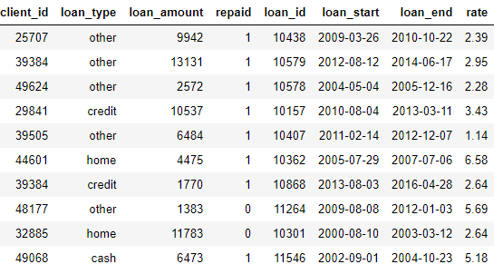
On the other hand, aggregations are performed across tables, and use a one-to-many relationship to group observations and then calculate statistics. For example, if we have another table with information on the loans of clients, where each client may have multiple loans, we can calculate statistics such as the average, maximum, and minimum of loans for each client.

This process involves grouping the loans table by the client, calculating the aggregations, and then merging the resulting data into the client data. Here’s how we would do that in Python using the language of Pandas.

These operations are not difficult by themselves, but if we have hundreds of variables spread across dozens of tables, this process is not feasible to do by hand. Ideally, we want a solution that can automatically perform transformations and aggregations across multiple tables and combine the resulting data into a single table. Although Pandas is a great resource, there’s only so much data manipulation we want to do by hand! (For more on manual feature engineering check out the excellent Python Data Science Handbook).

Featuretools

Fortunately, featuretools is exactly the solution we are looking for. This open-source Python library will automatically create many features from a set of related tables. Featuretools is based on a method known as “Deep Feature Synthesis”, which sounds a lot more imposing than it actually is (the name comes from stacking multiple features not because it uses deep learning!).

Deep feature synthesis stacks multiple transformation and aggregation operations (which are called feature primitives in the vocab of featuretools) to create features from data spread across many tables. Like most ideas in machine learning, it’s a complex method built on a foundation of simple concepts. By learning one building block at a time, we can form a good understanding of this powerful method.

First, let’s take a look at our example data. We already saw some of the dataset above, and the complete collection of tables is as follows:

• clients : basic information about clients at a credit union. Each client has only one row in this dataframe

** loans: loans made to the clients. Each loan has only own row in this dataframe but clients may have multiple loans.*

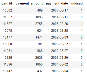
** payments: payments made on the loans. Each payment has only one row but each loan will have multiple payments.*

If we have a machine learning task, such as predicting whether a client will repay a future loan, we will want to combine all the information about clients into a single table. The tables are related (through the client_id and the loan_id variables) and we could use a series of transformations and aggregations to do this process by hand. However, we will shortly see that we can instead use featuretools to automate the process.

Entities and EntitySets

The first two concepts of featuretools are entities and entitysets. An entity is simply a table (or a DataFrame if you think in Pandas). An EntitySet is a collection of tables and the relationships between them. Think of an entityset as just another Python data structure, with its own methods and attributes.

We can create an empty entityset in featuretools using the following:

import featuretools as ft

# Create new entityset
es = ft.EntitySet(id = 'clients')

Now we have to add entities. Each entity must have an index, which is a column with all unique elements. That is, each value in the index must appear in the table only once. The index in the clients dataframe is the client_idbecause each client has only one row in this dataframe. We add an entity with an existing index to an entityset using the following syntax:

The loans dataframe also has a unique index, loan_id and the syntax to add this to the entityset is the same as for clients. However, for the payments dataframe, there is no unique index. When we add this entity to the entityset, we need to pass in the parameter make_index = True and specify the name of the index. Also, although featuretools will automatically infer the data type of each column in an entity, we can override this by passing in a dictionary of column types to the parameter variable_types .

For this dataframe, even though missed is an integer, this is not a numeric variable since it can only take on 2 discrete values, so we tell featuretools to treat is as a categorical variable. After adding the dataframes to the entityset, we inspect any of them:

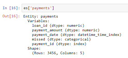The column types have been correctly inferred with the modification we specified. Next, we need to specify how the tables in the entityset are related.

Table Relationships

The best way to think of a relationship between two tables is the analogy of parent to child. This is a one-to-many relationship: each parent can have multiple children. In the realm of tables, a parent table has one row for every parent, but the child table may have multiple rows corresponding to multiple children of the same parent.

For example, in our dataset, the clients dataframe is a parent of the loans dataframe. Each client has only one row in clients but may have multiple rows in loans. Likewise, loans is the parent of payments because each loan will have multiple payments. The parents are linked to their children by a shared variable. When we perform aggregations, we group the child table by the parent variable and calculate statistics across the children of each parent.

To formalize a relationship in featuretools, we only need to specify the variable that links two tables together. The clients and the loans table are linked via the client_id variable and loans and payments are linked with the loan_id. The syntax for creating a relationship and adding it to the entityset are shown below:

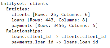The entityset now contains the three entities (tables) and the relationships that link these entities together. After adding entities and formalizing relationships, our entityset is complete and we are ready to make features.

Feature Primitives

Before we can quite get to deep feature synthesis, we need to understand feature primitives. We already know what these are, but we have just been calling them by different names! These are simply the basic operations that we use to form new features:

• Aggregations: operations completed across a parent-to-child (one-to-many) relationship that group by the parent and calculate stats for the children. An example is grouping the loan table by the client_id and finding the maximum loan amount for each client.
• Transformations: operations done on a single table to one or more columns. An example is taking the difference between two columns in one table or taking the absolute value of a column.

New features are created in featuretools using these primitives either by themselves or stacking multiple primitives. Below is a list of some of the feature primitives in featuretools (we can also define custom primitives):

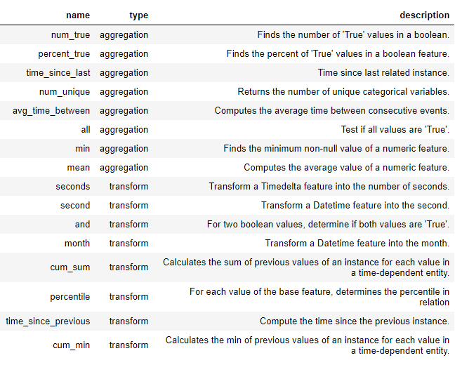Feature Primitives

These primitives can be used by themselves or combined to create features. To make features with specified primitives we use the ft.dfs function (standing for deep feature synthesis). We pass in the entityset, the target_entity , which is the table where we want to add the features, the selected trans_primitives (transformations), and agg_primitives (aggregations):

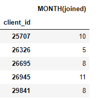
The result is a dataframe of new features for each client (because we made clients the target_entity). For example, we have the month each client joined which is a transformation feature primitive:

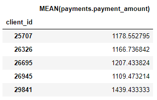
We also have a number of aggregation primitives such as the average payment amounts for each client:

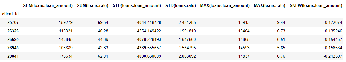
Even though we specified only a few feature primitives, featuretools created many new features by combining and stacking these primitives.

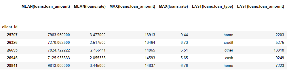The complete dataframe has 793 columns of new features!

Deep Feature Synthesis

We now have all the pieces in place to understand deep feature synthesis (dfs). In fact, we already performed dfs in the previous function call! A deep feature is simply a feature made of stacking multiple primitives and dfs is the name of process that makes these features. The depth of a deep feature is the number of primitives required to make the feature.

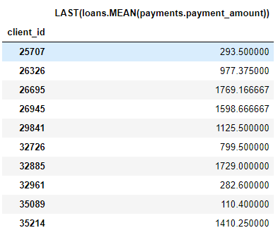
For example, the MEAN(payments.payment_amount) column is a deep feature with a depth of 1 because it was created using a single aggregation. A feature with a depth of two is LAST(loans(MEAN(payments.payment_amount)) This is made by stacking two aggregations: LAST (most recent) on top of MEAN. This represents the average payment size of the most recent loan for each client.

We can stack features to any depth we want, but in practice, I have never gone beyond a depth of 2. After this point, the features are difficult to interpret, but I encourage anyone interested to try “going deeper”.

We do not have to manually specify the feature primitives, but instead can let featuretools automatically choose features for us. To do this, we use the same ft.dfs function call but do not pass in any feature primitives:

Featuretools has built many new features for us to use. While this process does automatically create new features, it will not replace the data scientist because we still have to figure out what to do with all these features. For example, if our goal is to predict whether or not a client will repay a loan, we could look for the features most correlated with a specified outcome. Moreover, if we have domain knowledge, we can use that to choose specific feature primitives or seed deep feature synthesis with candidate features.

Next Steps

Automated feature engineering has solved one problem, but created another: too many features. Although it’s difficult to say before fitting a model which of these features will be important, it’s likely not all of them will be relevant to a task we want to train our model on. Moreover, having too many features can lead to poor model performance because the less useful features drown out those that are more important.

The problem of too many features is known as the curse of dimensionality. As the number of features increases (the dimension of the data grows) it becomes more and more difficult for a model to learn the mapping between features and targets. In fact, the amount of data needed for the model to perform well scales exponentially with the number of features.

The curse of dimensionality is combated with feature reduction (also known as feature selection): the process of removing irrelevant features. This can take on many forms: Principal Component Analysis (PCA), SelectKBest, using feature importances from a model, or auto-encoding using deep neural networks. However, feature reduction is a different topic for another article. For now, we know that we can use featuretools to create numerous features from many tables with minimal effort!

Conclusions

Like many topics in machine learning, automated feature engineering with featuretools is a complicated concept built on simple ideas. Using concepts of entitysets, entities, and relationships, featuretools can perform deep feature synthesis to create new features. Deep feature synthesis in turn stacks feature primitives — aggregations, which act across a one-to-many relationship between tables, and transformations, functions applied to one or more columns in a single table — to build new features from multiple tables.

In future articles, I’ll show how to use this technique on a real world problem, the Home Credit Default Risk competition currently being hosted on Kaggle. Stay tuned for that post, and in the meantime, read this introduction to get started in the competition! I hope that you can now use automated feature engineering as an aid in a data science pipeline. Our models are only as good as the data we give them, and automated feature engineering can help to make the feature creation process more efficient.

For more information on featuretools, including advanced usage, check out the online documentation. To see how featuretools is used in practice, read about the work of Feature Labs, the company behind the open-source library.

As always, I welcome feedback and constructive criticism and can be reached on Twitter @koehrsen_will.