
Automated Machine Learning Hyperparameter Tuning In Python

A complete walk through using Bayesian optimization for automated hyperparameter tuning in Python
Tuning machine learning hyperparameters is a tedious yet crucial task, as the performance of an algorithm can be highly dependent on the choice of hyperparameters. Manual tuning takes time away from important steps of the machine learning pipeline like feature engineering and interpreting results. Grid and random search are hands-off, but require long run times because they waste time evaluating unpromising areas of the search space. Increasingly, hyperparameter tuning is done by automated methods that aim to find optimal hyperparameters in less time using an informed search with no manual effort necessary beyond the initial set-up.
Bayesian optimization, a model-based method for finding the minimum of a function, has recently been applied to machine learning hyperparameter tuning, with results suggesting this approach can achieve better performance on the test set while requiring fewer iterations than random search. Moreover, there are now a number of Python libraries that make implementing Bayesian hyperparameter tuning simple for any machine learning model.
In this article, we will walk through a complete example of Bayesian hyperparameter tuning of a gradient boosting machine using the Hyperopt library. In an earlier article I outlined the concepts behind this method, so here we will stick to the implementation. Like with most machine learning topics, it’s not necessary to understand all the details, but knowing the basic idea can help you use the technique more effectively!
All the code for this article is available as a Jupyter Notebook on GitHub.
Table of Contents
- Bayesian Optimization Methods
- Four Parts of Optimization Problem
- Objective Function
- Domain Space
- Optimization Algorithm
- Result History
- Optimization
- Results
- Visualizing Search Results
- Evolution of Search
- Continue Searching
- Conclusions
Bayesian Optimization Methods
As a brief primer, Bayesian optimization finds the value that minimizes an objective function by building a surrogate function (probability model) based on past evaluation results of the objective. The surrogate is cheaper to optimize than the objective, so the next input values to evaluate are selected by applying a criterion to the surrogate (often Expected Improvement). Bayesian methods differ from random or grid search in that they use past evaluation results to choose the next values to evaluate. The concept is: limit expensive evaluations of the objective function by choosing the next input values based on those that have done well in the past.
In the case of hyperparameter optimization, the objective function is the validation error of a machine learning model using a set of hyperparameters. The aim is to find the hyperparameters that yield the lowest error on the validation set in the hope that these results generalize to the testing set. Evaluating the objective function is expensive because it requires training the machine learning model with a specific set of hyperparameters. Ideally, we want a method that can explore the search space while also limiting evaluations of poor hyperparameter choices. Bayesian hyperparameter tuning uses a continually updated probability model to “concentrate” on promising hyperparameters by reasoning from past results.
Python Options
There are several Bayesian optimization libraries in Python which differ in the algorithm for the surrogate of the objective function. In this article, we will work with Hyperopt, which uses the Tree Parzen Estimator (TPE) Other Python libraries include Spearmint (Gaussian Process surrogate) and SMAC (Random Forest Regression). There is a lot of interesting work going on in this area, so if you aren’t happy with one library, check out the alternatives! The general structure of a problem (which we will walk through here) translates between the libraries with only minor differences in syntax. For a basic introduction to Hyperopt, see this article.
Four Parts of Optimization Problem
There are four parts to a Bayesian Optimization problem:
- Objective Function: what we want to minimize, in this case the validation error of a machine learning model with respect to the hyperparameters
- Domain Space: hyperparametervalues to search over
- Optimization algorithm: method for constructing the surrogate model and choosing the next hyperparameter values to evaluate
- Result history: stored outcomes from evaluations of the objective function consisting of the hyperparameters and validation loss
With those four pieces, we can optimize (find the minimum) of any function that returns a real value. This is a powerful abstraction that lets us solve many problems in addition to tuning machine learning hyperparameters.
Dataset
For this example, we will use the Caravan Insurance dataset where the objective is to predict whether a customer will purchase an insurance policy. This is a supervised classification problem with 5800 training observations and 4000 testing points. The metric we will use to assess performance is the Receiver Operating Characteristic Area Under the Curve (ROC AUC) because this is an imbalanced classification problem. (A higher ROC AUC is better with a score of 1 indicating a perfect model). The dataset is shown below:
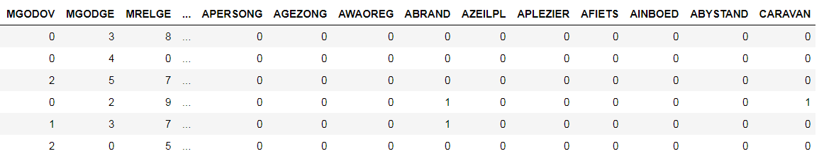 Dataset (CARAVAN) is the label
Because Hyperopt requires a value to minimize, we will return 1-ROC AUC from the objective function, thereby driving up the ROC AUC.
Gradient Boosting Model
Detailed knowledge of the gradient boosting machine (GBM) is not necessary for this article and here are the basics we need to understand: The GBM is an ensemble boosting method based on using weak learners (almost always decision trees) trained sequentially to form a strong model. There are many hyperparameters in a GBM controlling both the entire ensemble and individual decision trees. One of the most effective methods for choosing the number of trees (called estimators) is early stopping which we will use. LightGBM provides a fast and simple implementation of the GBM in Python.
For more details on the GBM, here’s a high level article and a technical paper.
With the necessary background out of the way, let’s go through writing the four parts of a Bayesian optimization problem for hyperparameter tuning.
Objective Function
The objective function is what we are trying to minimize. It takes in a set of values — in this case hyperparameters for the GBM — and outputs a real value to minimize — the cross validation loss. Hyperopt treats the objective function as a black box because it only considers what goes in and what comes out. The algorithm does not need to know the internals of the objective function in order to find the input values that minimize the loss! At a very high level (in pseudocode), our objective function should be:
def objective(hyperparameters):
    """Returns validation score from hyperparameters"""

    model = Classifier(hyperparameters)
    validation_loss = cross_validation(model, training_data)

    return validation_loss
We need to be careful not to use the loss on the testing set because we can only use the testing set a single time, when we evaluate the final model. Instead, we evaluate the hyperparameters on a validation set. Moreover, rather than separating training data into a distinct validation set, we use KFold cross validation, which, in addition to preserving valuable training data, should give us a less biased estimate of error on the testing set.
The basic structure of the objective function for hyperparameter tuning will be the same across models: the function takes in the hyperparameters and returns the cross-validation error using those hyperparameters. Although this example is specific to the GBM, the structure can be applied to other methods.
The complete objective function for the Gradient Boosting Machine using 10 fold cross validation with early stopping is shown below.
The main line is cv_results = lgb.cv(...) . To implement cross-validation with early stopping , we use the LightGBM function cv which takes in the hyperparameters, a training set, a number of folds to use for cross validation, and several other arguments. We set the number of estimators ( num_boost_round) to 10000, but this number won’t actually be reached because we are using early_stopping_rounds to stop the training when validation scores have not improved for 100 estimators. Early stopping is an effective method for choosing the number of estimators rather than setting this as another hyperparameter that needs to be tuned!
Once the cross validation is complete, we get the best score (ROC AUC), and then, because we want a value to minimize, we take 1-best score. This value is then returned as the loss key in the return dictionary.
This is objective function is actually a little more complicated than it needs to be because we return a dictionary of values. For the objective function in Hyperopt, we can either return a single value, the loss, or a dict that has at a minimum keys "loss" and "status" . Returning the hyperparameters will let us inspect the loss resulting from each set of hyperparameters.
Domain Space
The domain space represents the range of values we want to evaluate for each hyperparameter. Each iteration of the search, the Bayesian optimization algorithm will choose one value for each hyperparameter from the domain space. When we do random or grid search, the domain space is a grid. In Bayesian optimization the idea is the same except this space has probability distributions for each hyperparameter rather than discrete values.
Specifying the domain is the trickiest part of a Bayesian optimization problem. If we have experience with a machine learning method, we can use it to inform our choices of hyperparameter distributions by placing greater probability where we think the best values are. However, the optimal model settings will vary between datasets and with a high-dimensionality problem (many hyperparameters) it can be difficult to figure out the interaction between hyperparameters. In cases where we aren’t sure about the best values, we can use wide distributions and let the Bayesian algorithm do the reasoning for us.
First, we should look at all the hyperparameters in a GBM:
import lgb

# Default gradient boosting machine classifier
model = lgb.LGBMClassifier()
model

**LGBMClassifier(boosting_type='gbdt', n_estimators=100,
               class_weight=None, colsample_bytree=1.0,
               learning_rate=0.1, max_depth=-1,
               min_child_samples=20,
               min_child_weight=0.001, min_split_gain=0.0,
               n_jobs=-1, num_leaves=31, objective=None,
               random_state=None, reg_alpha=0.0, reg_lambda=0.0,
               silent=True, subsample=1.0,
               subsample_for_bin=200000, subsample_freq=1)**
I’m not sure there’s anyone in the world who knows how all of these interact together! Some of these we don’t have to tune (such as objective and random_state ) and we will use early stopping to find the best n_estimators. However, we still have 10 hyperparameters to optimize! When first tuning a model, I usually create a wide domain space centered around the default values and then refine it in subsequent searches.
As an example, let’s define a simple domain in Hyperopt, a discrete uniform distribution for the number of leaves in each tree in the GBM:
from hyperopt import hp

# Discrete uniform distribution
num_leaves = {'num_leaves': hp.quniform('num_leaves', 30, 150, 1)}
This is a discrete uniform distribution because the number of leaves must be an integer (discrete) and each value in the domain is equally likely (uniform).
Another choice of distribution is the log uniform which distributes values evenly on a logarithmic scale. We will use a log uniform (from 0.005 to 0.2) for the learning rate because it varies across several orders of magnitude:
# Learning rate log uniform distribution
learning_rate = {'learning_rate': hp.loguniform('learning_rate',
                                                 np.log(0.005),
                                                 np.log(0.2)}
Because this is a log-uniform distribution, the values are drawn between exp(low) and exp(high). The plot on the left below shows the discrete uniform distribution and the plot on the right is the log uniform. These are kernel density estimate plots so the y-axis is density and not a count!
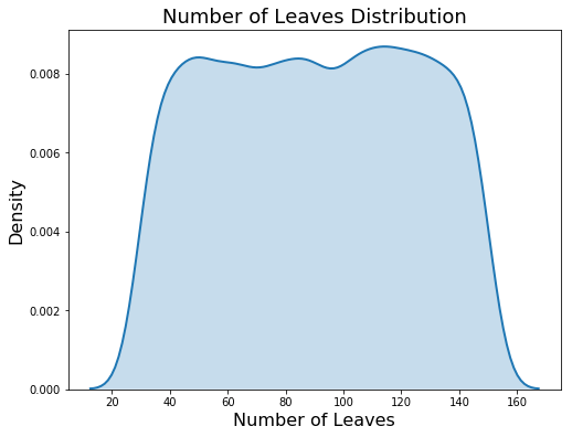
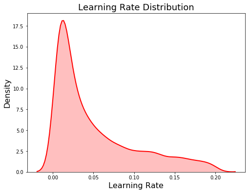 Domain for num_leaves (left) and learning_rate (right)
Now, let’s define the entire domain:
Here we use a number of different domain distribution types:
choice: categorical variablesquniform: discrete uniform (integers spaced evenly)uniform: continuous uniform (floats spaced evenly)loguniform: continuous log uniform (floats spaced evenly on a log scale)
(There are other distributions as well listed in the documentation.)
There is one important point to notice when we define the boosting type:
Here we are using a conditional domain which means the value of one hyperparameter depends on the value of another. For the boosting type "goss", the gbm cannot use subsampling (selecting only a [subsample](https://astro.temple.edu/~msobel/courses_files/StochasticBoosting(gradient).pdf?) fraction of the training observations to use on each iteration). Therefore, the subsample ratio is set to 1.0 (no subsampling) if the boosting type is "goss" but is 0.5–1.0 otherwise. This is implemented using a nested domain.
Conditional nesting can be useful when we are using different machine learning models with completely separate parameters. A conditional lets us use different sets of hyperparameters depending on the value of a choice.
Now that our domain is defined, we can draw one example from it to see what a typical sample looks like. When we sample, because subsample is initially nested, we need to assign it to a top-level key. This is done using the Python dictionary get method with a default value of 1.0.
**{'boosting_type': 'gbdt',
 'class_weight': 'balanced',
 'colsample_bytree': 0.8111305579351727,
 'learning_rate': 0.16186471096789776,
 'min_child_samples': 470.0,
 'num_leaves': 88.0,
 'reg_alpha': 0.6338327001528129,
 'reg_lambda': 0.8554826167886239,
 'subsample_for_bin': 280000.0,
 'subsample': 0.6318665053932255}**
(This reassigning of nested keys is necessary because the gradient boosting machine cannot deal with nested hyperparameter dictionaries).
Optimization Algorithm
Although this is the most conceptually difficult part of Bayesian Optimization, creating the optimization algorithm in Hyperopt is a single line. To use the Tree Parzen Estimator the code is:
from hyperopt import tpe

# Algorithm
tpe_algorithm = tpe.suggest
That’s all there is to it! Hyperopt only has the TPE option along with random search, although the GitHub page says other methods may be coming. During optimization, the TPE algorithm constructs the probability model from the past results and decides the next set of hyperparameters to evaluate in the objective function by maximizing the expected improvement.
Result History
Keeping track of the results is not strictly necessary as Hyperopt will do this internally for the algorithm. However, if we want to find out what is going on behind the scenes, we can use a Trials object which will store basic training information and also the dictionary returned from the objective function (which includes the loss andparams ). Making a trials object is one line:
from hyperopt import Trials

# Trials object to track progress
bayes_trials = Trials()
Another option which will allow us to monitor the progress of a long training run is to write a line to a csv file with each search iteration. This also saves all the results to disk in case something catastrophic happens and we lose the trials object (speaking from experience). We can do this using the csv library. Before training we open a new csv file and write the headers:
and then within the objective function we can add lines to write to the csv on every iteration (the complete objective function is in the notebook):
Writing to a csv means we can check the progress by opening the file while training (although not in Excel because this will cause an error in Python. Use tail out_file.csv from bash to view the last rows of the file).
Optimization
Once we have the four parts in place, optimization is run with fmin :
Each iteration, the algorithm chooses new hyperparameter values from the surrogate function which is constructed based on the previous results and evaluates these values in the objective function. This continues for MAX_EVALS evaluations of the objective function with the surrogate function continually updated with each new result.
Results
The best object that is returned from fmin contains the hyperparameters that yielded the lowest loss on the objective function:
**{'boosting_type': 'gbdt',
   'class_weight': 'balanced',
   'colsample_bytree': 0.7125187075392453,
   'learning_rate': 0.022592570862044956,
   'min_child_samples': 250,
   'num_leaves': 49,
   'reg_alpha': 0.2035211643104735,
   'reg_lambda': 0.6455131715928091,
   'subsample': 0.983566228071919,
   'subsample_for_bin': 200000}**
Once we have these hyperparameters, we can use them to train a model on the full training data and then evaluate on the testing data (remember we can only use the test set once, when we evaluate the final model). For the number of estimators, we can use the number of estimators that returned the lowest loss in cross validation with early stopping. Final results are below:
**The best model scores 0.72506 AUC ROC on the test set.
The best cross validation score was 0.77101 AUC ROC.
This was achieved after 413 search iterations.**
As a reference, 500 iterations of random search returned a model that scored 0.7232 ROC AUC on the test set and 0.76850 in cross validation. A default model with no optimization scored 0.7143 ROC AUC on the test set.
There are a few important notes to keep in mind when we look at the results:
- The optimal hyperparameters are those that do best in cross validation and not necessarily those that do best on the testing data. When we use cross validation, we hope that these results generalize to the testing data.
- Even using 10-fold cross-validation, the hyperparameter tuning overfits to the training data. The best score from cross-validation is significantly higher than that on the testing data.
- Random search may return better hyperparameters just by sheer luck (re-running the notebook can change the results). Bayesian optimization is not guaranteed to find better hyperparameters and can get stuck in a local minimum of the objective function.
Bayesian optimization is effective, but it will not solve all our tuning problems. As the search progresses, the algorithm switches from exploration — trying new hyperparameter values — to exploitation — using hyperparameter values that resulted in the lowest objective function loss. If the algorithm finds a local minimum of the objective function, it might concentrate on hyperparameter values around the local minimum rather than trying different values located far away in the domain space. Random search does not suffer from this issue because it does not concentrate on any values!
Another important point is that the benefits of hyperparameter optimization will differ with the dataset. This is a relatively small dataset (~ 6000 training observations) and there is a small payback to tuning the hyperparameters (getting more data would be a better use of time!). With all of those caveats in mind, in this case, with Bayesian optimization we can get:
- Better performance on the testing set
- Fewer iterations to tune the hyperparameters
Bayesian methods can (although will not always) yield better tuning results than random search. In the next few sections, we will examine the evolution of the Bayesian hyperparameter search and compare to random search to understand how Bayesian Optimization works.
Visualizing Search Results
Graphing the results is an intuitive way to understand what happens during the hyperparameter search. Moreover, it’s helpful to compare Bayesian Optimization to random search so we can see how the methods differ. To see how the plots are made and random search is implemented, see the notebook, but here we will go through the results. (As a note, the exact results will change across iterations, so if you run the notebook, don’t be surprised if you get different images. All of these plots are made with 500 iterations).
First we can make a kernel density estimate plot of the learning_rate sampled in random search and Bayes Optimization. As a reference, we can also show the sampling distribution. The vertical dashed lines show the best values (according to cross validation) for the learning rate.
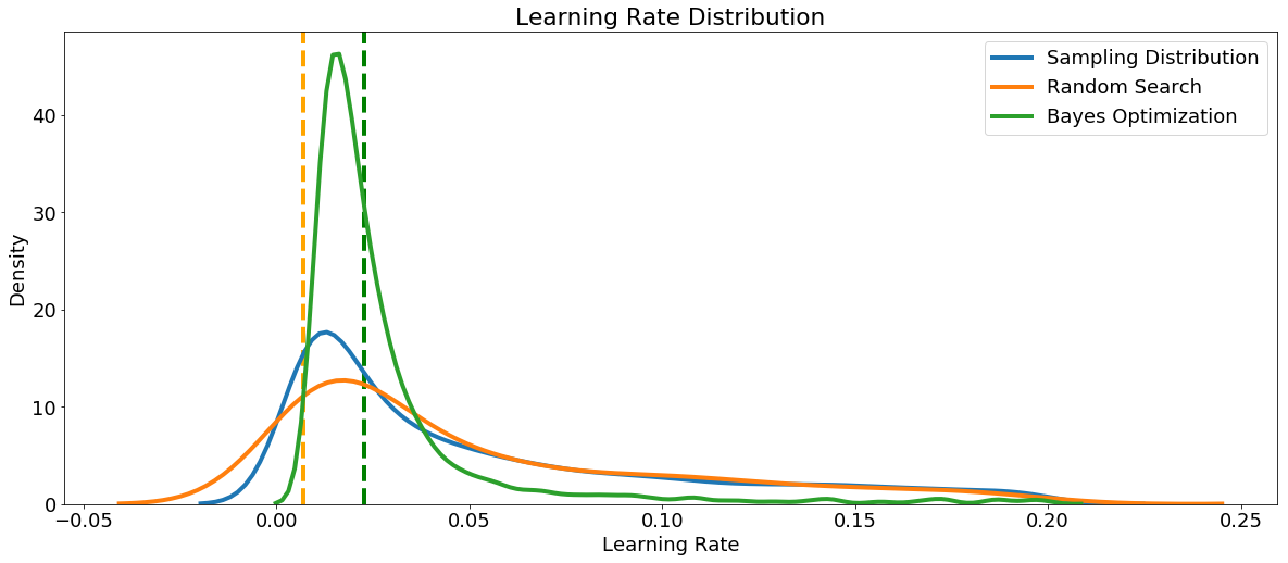 We defined the learning rate as a log-normal between 0.005 and 0.2, and the Bayesian Optimization results look similar to the sampling distribution. This tells us that the distribution we defined looks to be appropriate for the task, although the optimal value is a little higher than where we placed the greatest probability. This could be used to inform the domain for further searches.
Another hyperparameter is the boosting type, with the bar plots of each type evaluated during random search and Bayes optimization shown below. Since random search does not pay attention to past results, we would expect each boosting type to be used roughly the same number of times.
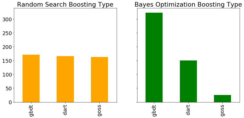 According to the Bayesian algorithm, the
 gdbt boosting type is more promising than dart or goss. Again, this could help inform further searches, either Bayesian methods or grid search. If we wanted to do a more informed grid search, we could use these results to define a smaller grid concentrated around the most promising values of the hyperparameters.
Since we have them, let’s look at all of the numeric hyperparameters from the reference distribution, random search, and Bayes Optimization. The vertical lines again indicate the best value of the hyperparameter for each search:

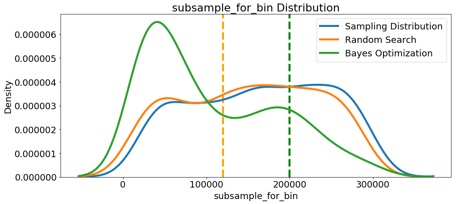
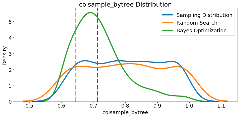
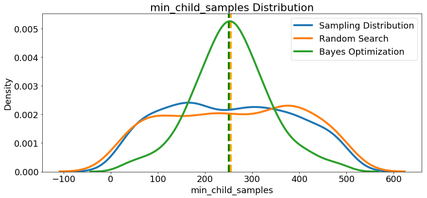
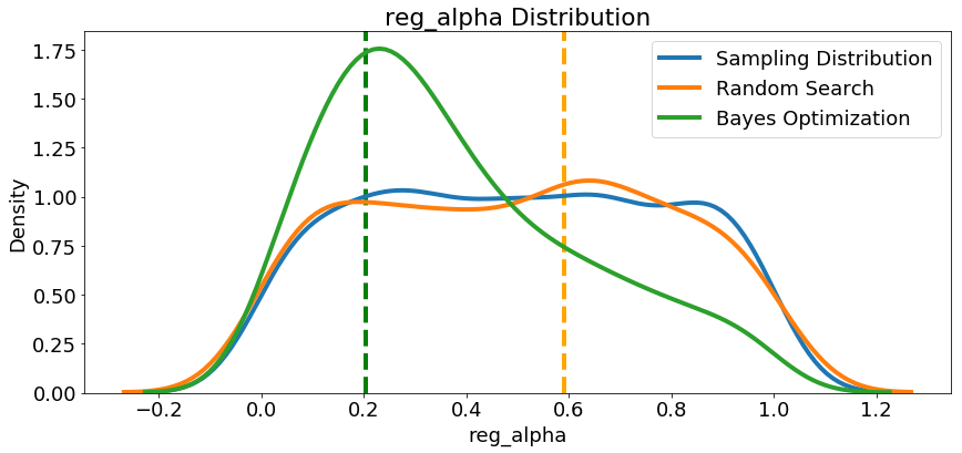
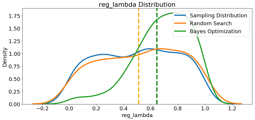 In most cases (except for the
 subsample_for_bin ) the Bayesian optimization search tends to concentrate (place more probability) near the hyperparameter values that yield the lowest loss in cross validation. This shows the fundamental idea of hyperparameter tuning using Bayesian methods: spend more time evaluating promising hyperparameter values.
There are also some interesting results here that might help us in the future when it comes time to define a domain space to search over. As just one example, it looks like reg_alpha and reg_lambda should complement one another: if one is high (close to 1.0), the other should be lower. There’s no guarantee this will hold across problems, but by studying the results, we can gain insights that might be applied to future machine learning problems!
Evolution of Search
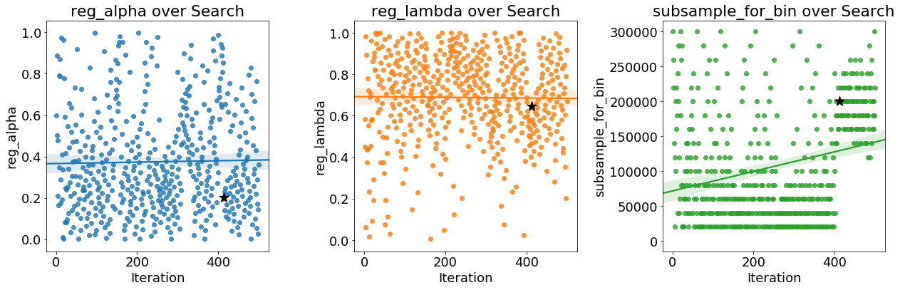
As the optimization progresses, we expect the Bayes method to focus on the more promising values of the hyperparameters: those that yield the lowest error in cross validation. We can plot the values of the hyperparameters versus the iteration to see if there are noticeable trends.
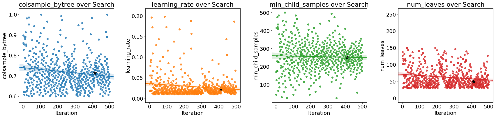 The black star indicates the optimal value. The
 colsample_bytree and learning_rate decrease over time which could guide us in future searches.
 Finally, if Bayes Optimization is working, we would expect the average validation score to increase over time (conversely the loss decreases):
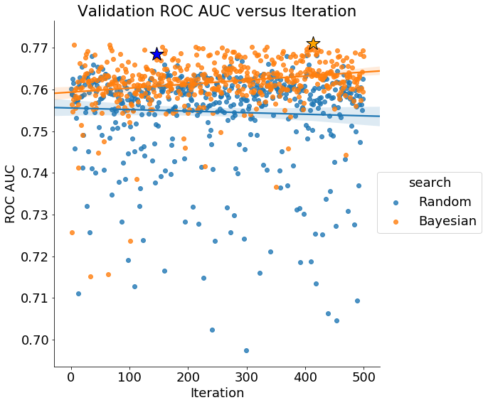 The validation scores from Bayesian hyperparameter optimization increase over time, indicating the method is trying “better” hyperparameter values (it should be noted that these are only better according to the validation score). Random search does not show an improvement over the iterations.
Continue Searching
If we are not satisfied with the performance of our model, we can keep searching using Hyperopt from where we left off. We just need to pass in the same trials object and the algorithm will continue searching.
As the algorithm progresses, it does more exploitation — picking values that have done well in the past — and less exploration — picking new values. Instead of continuing where the search left off, it might therefore be a good idea to start an entirely different search. If the best hyperparameters from the first search really are “optimal”, we would expect subsequent searches to focus on the same values. Given the high dimensionality of the problem, and the complex interactions between hyperparameters, it’s unlikely that another search would result in a similar set of hyperparameters.
After another 500 iterations of training, the final model scores 0.72736 ROC AUCon the test set. (We really should not have evaluated the first model on the test set and instead relied only on validation scores. The test set should ideally be used only once to get a measure of algorithm performance when deployed on new data). Again, this problem may have diminishing returns to further hyperparameter optimization because of the small size of the dataset and there will eventually be a plateau in validation error (there is an inherent limit to the performance of any model on a dataset because of hidden variables that are not measured and noisy data, referred to as Bayes’ Error).
Conclusions
Automated hyperparameter tuning of machine learning models can be accomplished using Bayesian optimization. In contrast to random search, Bayesian optimization chooses the next hyperparameters in an informed method to spend more time evaluating promising values. The end outcome can be fewer evaluations of the objective function and better generalization performance on the test set compared to random or grid search.
In this article, we walked step-by-step through Bayesian hyperparameter optimization in Python using Hyperopt. We were able to improve the test set performance of a Gradient Boosting Machine beyond both the baseline and random search although we need to be cautious of overfitting to the training data. Furthermore, we saw how random search differs from Bayesian Optimization by examining the resulting graphs which showed that the Bayesian method placed greater probability on the hyperparameter values that resulted in lower cross validation loss.
Using the four parts of an optimization problem, we can use Hyperopt to solve a wide variety of problems. The basic parts of Bayesian optimization also apply to a number of libraries in Python that implement different algorithms. Making the switch from manual to random or grid search is one small step, but to take your machine learning to the next level requires some automated form of hyperparameter tuning. Bayesian Optimization is one approach that is both easy to use in Python and can return better results than random search. Hopefully you now feel confident to start using this powerful method for your own machine learning problems!
As always, I welcome feedback and constructive criticism. I can be reached on Twitter @koehrsen_will.