
A Conceptual Explanation Of Bayesian Model Based Hyperparameter Optimization For Machine Learning

The concepts behind efficient hyperparameter tuning using Bayesian optimization
Following are four common methods of hyperparameter optimization for machine learning in order of increasing efficiency:
- Manual
- Grid search
- Random search
- Bayesian model-based optimization
(There are also other methods such as evolutionary and gradient-based.)
I was pretty proud that I’d recently moved up the ladder from manual to random search until I found this image deep in a paper by Bergstra et al.:
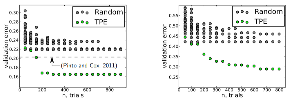 Validation Errors comparing random search and a model based approach on LFW (left) and PubFig83 (right)
These figures compare validation error for hyperparameter optimization of an image classification neural network with random search in grey and Bayesian Optimization (using the Tree Parzen Estimator or TPE) in green. Lower is better: a smaller validation set error generally means better test set performance, and a smaller number of trials means less time invested. Clearly, there are significant advantages to Bayesian methods, and these graphs, along with other impressive results, convinced me it was time to take the next step and learn model-based hyperparameter optimization.
The one-sentence summary of Bayesian hyperparameter optimization is: build a probability model of the objective function and use it to select the most promising hyperparameters to evaluate in the true objective function.
If you like to operate at a very high level, then this sentence may be all you need. However, if you want to understand the details, this article is my attempt to outline the concepts behind Bayesian optimization, in particular Sequential Model-Based Optimization (SMBO) with the Tree Parzen Estimator (TPE). With the mindset that you don’t know a concept until you can explain it to others, I went through several academic papers and will try to communicate the results in a (relatively) easy to understand format.
Although we can often implement machine learning methods without understanding how they work, I like to try and get an idea of what is going on so I can use the technique as effectively as possible. In later articles I’ll walk through using these methods in Python using libraries such as Hyperopt, so this article will lay the conceptual groundwork for implementations to come!
Update: Here is a brief Jupyter Notebook showing the basics of using Bayesian Model-Based Optimization in the Hyperopt Python library.
Hyperparameter Optimization
The aim of hyperparameter optimization in machine learning is to find the hyperparameters of a given machine learning algorithm that return the best performance as measured on a validation set. (Hyperparameters, in contrast to model parameters, are set by the machine learning engineer before training. The number of trees in a random forest is a hyperparameter while the weights in a neural network are model parameters learned during training. I like to think of hyperparameters as the model settings to be tuned.)
Hyperparameter optimization is represented in equation form as:
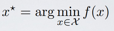 Here f(x) represents an objective score to minimize— such as RMSE or error rate— evaluated on the validation set; x is the set of hyperparameters that yields the lowest value of the score, and x can take on any value in the domain X. In simple terms, we want to find the model hyperparameters that yield the best score on the validation set metric.*
The problem with hyperparameter optimization is that evaluating the objective function to find the score is extremely expensive. Each time we try different hyperparameters, we have to train a model on the training data, make predictions on the validation data, and then calculate the validation metric. With a large number of hyperparameters and complex models such as ensembles or deep neural networks that can take days to train, this process quickly becomes intractable to do by hand!
Grid search and random search are slightly better than manual tuning because we set up a grid of model hyperparameters and run the train-predict -evaluate cycle automatically in a loop while we do more productive things (like feature engineering). However, even these methods are relatively inefficient because they do not choose the next hyperparameters to evaluate based on previous results. Grid and random search are completely uninformed by past evaluations, and as a result, often spend a significant amount of time evaluating “bad” hyperparameters.
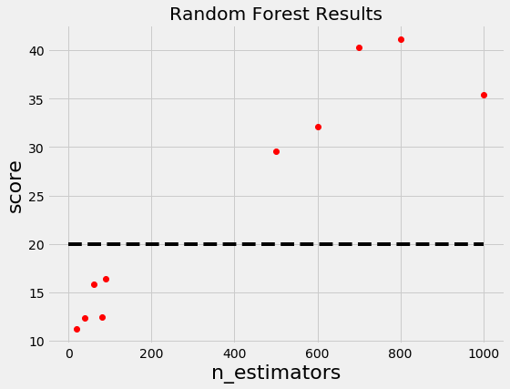
For example, if we have the following graph with a lower score being better, where does it make sense to concentrate our search? If you said below 200 estimators, then you already have the idea of Bayesian optimization! We want to focus on the most promising hyperparameters, and if we have a record of evaluations, then it makes sense to use this information for our next choice.
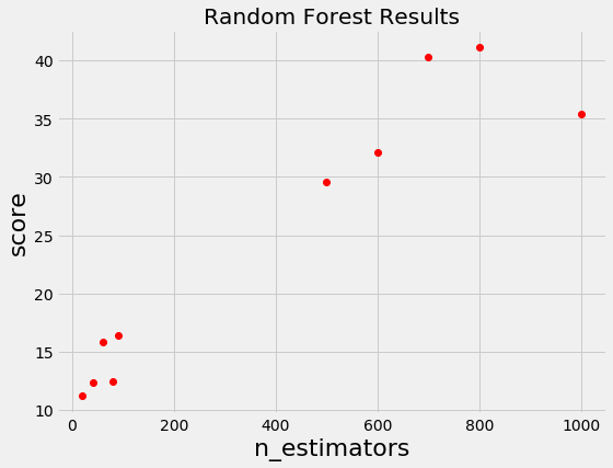 Random and grid search pay no attention to past results at all and would keep searching across the entire range of the number of estimators even though it’s clear the optimal answer (probably) lies in a small region!
Bayesian Optimization
Bayesian approaches, in contrast to random or grid search, keep track of past evaluation results which they use to form a probabilistic model mapping hyperparameters to a probability of a score on the objective function:
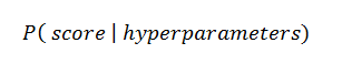 In the literature, this model is called a “surrogate” for the objective function and is represented as p(y | x). The surrogate is much easier to optimize than the objective function and Bayesian methods work by finding the next set of hyperparameters to evaluate on the actual objective function by selecting hyperparameters that perform best on the surrogate function. In other words:
- Build a surrogate probability model of the objective function
- Find the hyperparameters that perform best on the surrogate
- Apply these hyperparameters to the true objective function
- Update the surrogate model incorporating the new results
- Repeat steps 2–4 until max iterations or time is reached
The aim of Bayesian reasoning is to become “less wrong” with more data which these approaches do by continually updating the surrogate probability model after each evaluation of the objective function.
At a high-level, Bayesian optimization methods are efficient because they choose the next hyperparameters in an informed manner. The basic idea is: spend a little more time selecting the next hyperparameters in order to make fewer calls to the objective function. In practice, the time spent selecting the next hyperparameters is inconsequential compared to the time spent in the objective function. By evaluating hyperparameters that appear more promising from past results, Bayesian methods can find better model settings than random search in fewer iterations.
If there’s one thing to take away from this article it’s that Bayesian model-based methods can find better hyperparameters in less time because they reason about the best set of hyperparameters to evaluate based on past trials.
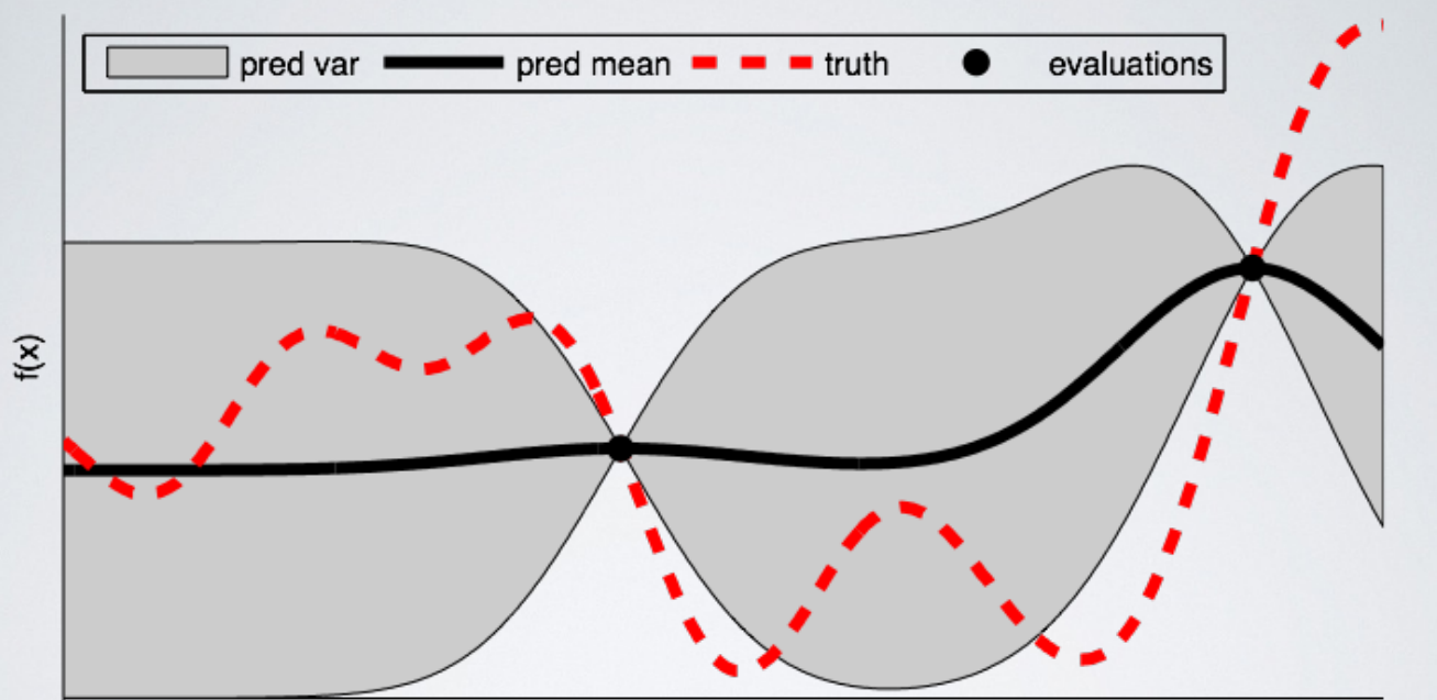
As a good visual description of what is occurring in Bayesian Optimization take a look at the images below (source). The first shows an initial estimate of the surrogate model — in black with associated uncertainty in gray — after two evaluations. Clearly, the surrogate model is a poor approximation of the actual objective function in red:
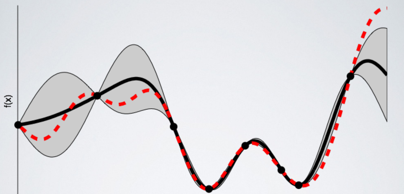
 The next image shows the surrogate function after 8 evaluations. Now the surrogate almost exactly matches the true function. Therefore, if the algorithm selects the hyperparameters that maximize the surrogate, they will likely yield very good results on the true evaluation function.
 Bayesian methods have always made sense to me because they operate in much the same way we do: we form an initial view of the world (called a prior) and then we update our model based on new experiences (the updated model is called a posterior). Bayesian hyperparameter optimization takes that framework and applies it to finding the best value of model settings!
Sequential Model-Based Optimization
Sequential model-based optimization (SMBO) methods (SMBO) are a formalization of Bayesian optimization. The sequential refers to running trials one after another, each time trying better hyperparameters by applying Bayesian reasoning and updating a probability model (surrogate).
There are five aspects of model-based hyperparameter optimization:
- A domain of hyperparameters over which to search
- An objective function which takes in hyperparameters and outputs a score that we want to minimize (or maximize)
- The surrogate model of the objective function
- A criteria, called a selection function, for evaluating which hyperparameters to choose next from the surrogate model
- A history consisting of (score, hyperparameter) pairs used by the algorithm to update the surrogate model
There are several variants of SMBO methods that differ in steps 3–4, namely, how they build a surrogate of the objective function and the criteria used to select the next hyperparameters. Several common choices for the surrogate model are Gaussian Processes, Random Forest Regressions, and Tree Parzen Estimators (TPE) while the most common choice for step 4 is Expected Improvement. In this post, we will focus on TPE and Expected Improvement.
Domain
In the case of random search and grid search, the domain of hyperparameters we search is a grid. An example for a random forest is shown below:
For a model-based approach, the domain consists of probability distributions. As with a grid, this lets us encode domain knowledge into the search process by placing greater probability in regions where we think the true best hyperparameters lie. If we wanted to express the above grid as a probability distribution, it may look something like this:
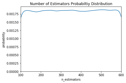
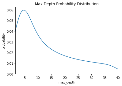
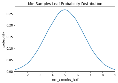 Here we have a uniform, log-normal, and normal distribution. These are informed by prior practice/knowledge (for example the learning rate domain is usually a log-normal distribution over several orders of magnitude).
Objective Function
The objective function takes in hyperparameters and outputs a single real-valued score that we want to minimize (or maximize). As an example, let’s consider the case of building a random forest for a regression problem. The hyperparameters we want to optimize are shown in the hyperparameter grid above and the score to minimize is the Root Mean Squared Error. Our objective function would then look like (in Python):
While the objective function looks simple, it is very expensive to compute! If the objective function could be quickly calculated, then we could try every single possible hyperparameter combination (like in grid search). If we are using a simple model, a small hyperparameter grid, and a small dataset, then this might be the best way to go. However, in cases where the objective function may take hours or even days to evaluate, we want to limit calls to it.
The entire concept of Bayesian model-based optimization is to reduce the number of times the objective function needs to be run by choosing only the most promising set of hyperparameters to evaluate based on previous calls to the evaluation function. The next set of hyperparameters are selected based on a model of the objective function called a surrogate.
Surrogate Function (Probability Model)
The surrogate function, also called the response surface, is the probability representation of the objective function built using previous evaluations. This is called sometimes called a response surface because it is a high-dimensional mapping of hyperparameters to the probability of a score on the objective function. Below is a simple example with only two hyperparameters:
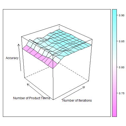 Response surface for AdaBoost algorithm (Source)
There are several different forms of the surrogate function including Gaussian Processes and Random Forest regression. However, in this post we will focus on the Tree-structured Parzen Estimator as put forward by Bergstra et al in the paper “Algorithms for Hyper-Parameter Optimization”. These methods differ in how they construct the surrogate function which we’ll explain in just a bit. First we need to talk about the selection function.
Selection Function
The selection function is the criteria by which the next set of hyperparameters are chosen from the surrogate function. The most common choice of criteria is Expected Improvement:
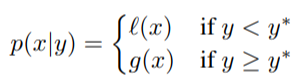
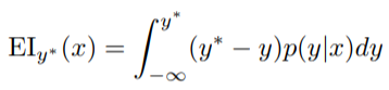 Here y is a threshold value of the objective function, x is the proposed set of hyperparameters, y is the actual value of the objective function using hyperparameters x, and p(y | x) is the surrogate probability model expressing the probability of y given x. If that’s all a little much, in simpler terms, the aim is to maximize the Expected Improvement with respect to x. This means finding the best hyperparameters under the surrogate function p (y | x).*
| If p (y | x) is zero everywhere that y < y*, then the hyperparameters x are not expected to yield any improvement. If the integral is positive, then it means that the hyperparameters x are expected to yield a better result than the threshold value. |
Tree-structured Parzen Estimator (TPE)
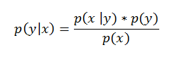
| Now let’s get back to the surrogate function. The methods of SMBO differ in how they construct the surrogate model p(y | x). The Tree-structured Parzen Estimator builds a model by applying Bayes rule. Instead of directly representing p( y | x), it instead uses: |
 Bayes Rule in Action!
| p (x | y), which is the probability of the hyperparameters given the score on the objective function, in turn is expressed: |
 where y < y represents a lower value of the objective function than the threshold. The explanation of this equation is that we make two different distributions for the hyperparameters: one where the value of the objective function is less than the threshold, l(x), and one where the value of the objective function is greater than the threshold, g(x).*
Let’s update our Random Forest graph to include a threshold:
 Now we construct two probability distributions for the number of estimators, one using the estimators that yielded values under the threshold and one using the estimators that yielded values above the threshold.
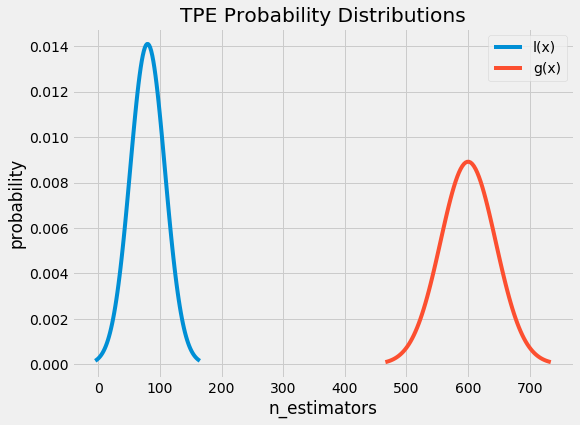 Intuitively, it seems that we want to draw values of x from _l(x)_ and not from _g(x)_ because this distribution is based only on values of x that yielded lower scores than the threshold. It turns out this is exactly what the math says as well! With Bayes Rule, and a few substitutions, the expected improvement equation (which we are trying to maximize) becomes:
 The term on the far right is the most important part. What this says is that the Expected Improvement is proportional to the ratio _l(x) / g(x)_ and therefore, to maximize the Expected Improvement, we should maximize this ratio. Our intuition was correct: we should draw values of the hyperparameters which are more likely under _l(x)_ than under _g(x)_!
The Tree-structured Parzen Estimator works by drawing sample hyperparameters from l(x), evaluating them in terms of l(x) / g(x), and returning the set that yields the highest value under l(x) / g(x) corresponding to the greatest expected improvement_._ These hyperparameters are then evaluated on the objective function. If the surrogate function is correct, then these hyperparameters should yield a better value when evaluated!
The expected improvement criteria allows the model to balance exploration versus exploitation. l(x) is a distribution and not a single value which means that the hyperparameters drawn are likely close but not exactly at the maximum of the expected improvement. Moreover, because the surrogate is just an estimate of the objective function, the selected hyperparameters may not actually yield an improvement when evaluated and the surrogate model will have to be updated. This updating is done based on the current surrogate model and the history of objective function evaluations.
History
Each time the algorithm proposes a new set of candidate hyperparameters, it evaluates them with the actual objective function and records the result in a pair (score, hyperparameters). These records form the history. The algorithm builds l(x) and g(x) using the history to come up with a probability model of the objective function that improves with each iteration.
This is Bayes’ Rule at work: we have an initial estimate for the surrogate of the objective function that we update as we gather more evidence. Eventually, with enough evaluations of the objective function, we hope that our model accurately reflects the objective function and the hyperparameters that yield the greatest Expected Improvement correspond to the hyperparameters that maximize the objective function.
Putting it All Together
How do Sequential Model-Based Methods help us more efficiently search the hyperparameter space? Because the algorithm is proposing better candidate hyperparameters for evaluation, the score on the objective function improves much more rapidly than with random or grid search leading to fewer overall evaluations of the objective function.
Even though the algorithm spends more time selecting the next hyperparameters by maximizing the Expected Improvement, this is much cheaper in terms of computational cost than evaluating the objective function. In a paper about using SMBO with TPE, the authors reported that finding the next proposed set of candidate hyperparameters took several seconds, while evaluating the actual objective function took hours.
If we are using better-informed methods to choose the next hyperparameters, that means we can spend less time evaluating poor hyperparameter choices. Furthermore, sequential model-based optimization using tree-structured Parzen estimators is able to find better hyperparameters than random search in the same number of trials. In other words, we get
- Reduced running time of hyperparameter tuning
- Better scores on the testing set
Hopefully, this has convinced you Bayesian model-based optimization is a technique worth trying!
Implementation
Fortunately for us, there are now a number of libraries that can do SMBO in Python. Spearmint and MOE use a Gaussian Process for the surrogate, Hyperopt uses the Tree-structured Parzen Estimator, and SMAC uses a Random Forest regression. These libraries all use the Expected Improvement criterion to select the next hyperparameters from the surrogate model. In later articles we will take a look at using Hyperopt in Python and there are already several good articles and code examples for learning.
Conclusions
Bayesian model-based optimization methods build a probability model of the objective function to propose smarter choices for the next set of hyperparameters to evaluate. SMBO is a formalization of Bayesian optimization which is more efficient at finding the best hyperparameters for a machine learning model than random or grid search.
Sequential model-based optimization methods differ in they build the surrogate, but they all rely on information from previous trials to propose better hyperparameters for the next evaluation. The Tree Parzen Estimator is one algorithm that uses Bayesian reasoning to construct the surrogate model and can select the next hyperparameters using Expected Improvement.
There are a number of libraries to implement SMBO in Python which we will explore in further articles. The concepts are a little tough at first, but understanding them will allow us to use the tools built on them more effectively. I’d like to mention I’m still trying to work my way through the details and if I’ve made a mistake, please let me know (civilly)!
For more details, the following articles are extremely helpful:
- Algorithms for Hyper-Parameter Optimization [Link]
- Making a Science of Model Search: Hyperparameter Optimization in Hundreds of Dimensions for Vision Architectures [Link]
- Bayesian Optimization Primer [Link]
- Taking the Human Out of the Loop: A Review of Bayesian Optimization [Link]
As always, I welcome feedback and constructive criticism. I can be reached on Twitter @koehrsen_will