
Introduction To Bayesian Linear Regression

An explanation of the Bayesian approach to linear modeling
The Bayesian vs Frequentist debate is one of those academic arguments that I find more interesting to watch than engage in. Rather than enthusiastically jump in on one side, I think it’s more productive to learn both methods of statistical inference and apply them where appropriate. In that line of thinking, recently, I have been working to learn and apply Bayesian inference methods to supplement the frequentist statistics covered in my grad classes.
One of my first areas of focus in applied Bayesian Inference was Bayesian Linear modeling. The most important part of the learning process might just be explaining an idea to others, and this post is my attempt to introduce the concept of Bayesian Linear Regression. We’ll do a brief review of the frequentist approach to linear regression, introduce the Bayesian interpretation, and look at some results applied to a simple dataset. I kept the code out of this article, but it can be found on GitHub in a Jupyter Notebook.
Recap of Frequentist Linear Regression
The frequentist view of linear regression is probably the one you are familiar with from school: the model assumes that the response variable (y) is a linear combination of weights multiplied by a set of predictor variables (x). The full formula also includes an error term to account for random sampling noise. For example, if we have two predictors, the equation is:
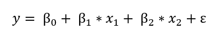 y is the response variable (also called the dependent variable), β’s are the weights (known as the model parameters), x’s are the values of the predictor variables, and ε is an error term representing random sampling noise or the effect of variables not included in the model.
Linear Regression is a simple model which makes it easily interpretable: β_0 is the intercept term and the other weights, β’s, show the effect on the response of increasing a predictor variable. For example, if β_1 is 1.2, then for every unit increase in x_1,the response will increase by 1.2.
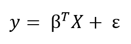
We can generalize the linear model to any number of predictors using matrix equations. Adding a constant term of 1 to the predictor matrix to account for the intercept, we can write the matrix formula as:
 The goal of learning a linear model from training data is to find the coefficients, β, that best explain the data. In frequentist linear regression, the best explanation is taken to mean the coefficients, β, that minimize the residual sum of squares (RSS). RSS is the total of the squared differences between the known values (y) and the predicted model outputs (ŷ, pronounced y-hat indicating an estimate). The residual sum of squares is a function of the model parameters:
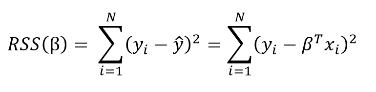 The summation is taken over the N data points in the training set. We won’t go into the details here (check out this reference for the derivation), but this equation has a closed form solution for the model parameters, β, that minimize the error. This is known as the maximum likelihood estimate of β because it is the value that is the most probable given the inputs, X, and outputs, y. The closed form solution expressed in matrix form is:
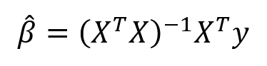 (Again, we have to put the ‘hat’ on β because it represents an estimate for the model parameters.) Don’t let the matrix math scare you off! Thanks to libraries like Scikit-learn in Python, we generally don’t have to calculate this by hand (although it is good practice to code a linear regression). This method of fitting the model parameters by minimizing the RSS is called Ordinary Least Squares (OLS).
What we obtain from frequentist linear regression is a single estimate for the model parameters based only on the training data. Our model is completely informed by the data: in this view, everything that we need to know for our model is encoded in the training data we have available.
Once we have β-hat, we can estimate the output value of any new data point by applying our model equation:
 As an example of OLS, we can perform a linear regression on real-world data which has duration and calories burned for 15000 exercise observations. Below is the data and OLS model obtained by solving the above matrix equation for the model parameters:
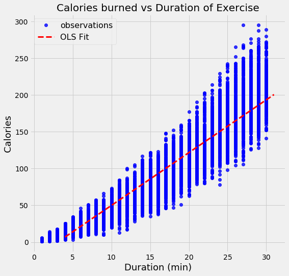 With OLS, we get a _single_ estimate of the model parameters, in this case, the intercept and slope of the line.We can write the equation produced by OLS:
calories = -21.83 + 7.17 * duration
From the slope, we can say that every additional minute of exercise results in 7.17 additional calories burned. The intercept in this case is not as helpful, because it tells us that if we exercise for 0 minutes, we will burn -21.86 calories! This is just an artifact of the OLS fitting procedure, which finds the line that minimizes the error on the training data regardless of whether it physically makes sense.
If we have a new datapoint, say an exercise duration of 15.5 minutes, we can plug it into the equation to get a point estimate of calories burned:
calories = -21.83 + 7.17 * 15.5 = 89.2
Ordinary least squares gives us a single point estimate for the output, which we can interpret as the most likely estimate given the data. However, if we have a small dataset we might like to express our estimate as a distribution of possible values. This is where Bayesian Linear Regression comes in.
Bayesian Linear Regression
In the Bayesian viewpoint, we formulate linear regression using probability distributions rather than point estimates. The response, y, is not estimated as a single value, but is assumed to be drawn from a probability distribution. The model for Bayesian Linear Regression with the response sampled from a normal distribution is:
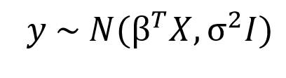 The output, y is generated from a normal (Gaussian) Distribution characterized by a mean and variance. The mean for linear regression is the transpose of the weight matrix multiplied by the predictor matrix. The variance is the square of the standard deviation σ (multiplied by the Identity matrix because this is a multi-dimensional formulation of the model).
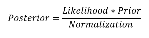
The aim of Bayesian Linear Regression is not to find the single “best” value of the model parameters, but rather to determine the posterior distribution for the model parameters. Not only is the response generated from a probability distribution, but the model parameters are assumed to come from a distribution as well. The posterior probability of the model parameters is conditional upon the training inputs and outputs:
![]() Here, P(β|y, X) is the posterior probability distribution of the model parameters given the inputs and outputs. This is equal to the likelihood of the data, P(y|β, X), multiplied by the prior probability of the parameters and divided by a normalization constant. This is a simple expression of Bayes Theorem, the fundamental underpinning of Bayesian Inference:
Here, P(β|y, X) is the posterior probability distribution of the model parameters given the inputs and outputs. This is equal to the likelihood of the data, P(y|β, X), multiplied by the prior probability of the parameters and divided by a normalization constant. This is a simple expression of Bayes Theorem, the fundamental underpinning of Bayesian Inference:
 Let’s stop and think about what this means. In contrast to OLS, we have a posterior _distribution_ for the model parameters that is proportional to the likelihood of the data multiplied by the _prior_ probability of the parameters. Here we can observe the two primary benefits of Bayesian Linear Regression.
- Priors: If we have domain knowledge, or a guess for what the model parameters should be, we can include them in our model, unlike in the frequentist approach which assumes everything there is to know about the parameters comes from the data. If we don’t have any estimates ahead of time, we can use non-informative priors for the parameters such as a normal distribution.
- Posterior: The result of performing Bayesian Linear Regression is a distribution of possible model parameters based on the data and the prior. This allows us to quantify our uncertainty about the model: if we have fewer data points, the posterior distribution will be more spread out.
As the amount of data points increases, the likelihood washes out the prior, and in the case of infinite data, the outputs for the parameters converge to the values obtained from OLS.
The formulation of model parameters as distributions encapsulates the Bayesian worldview: we start out with an initial estimate, our prior, and as we gather more evidence, our model becomes less wrong. Bayesian reasoning is a natural extension of our intuition. Often, we have an initial hypothesis, and as we collect data that either supports or disproves our ideas, we change our model of the world (ideally this is how we would reason)!
Implementing Bayesian Linear Regression
In practice, evaluating the posterior distribution for the model parameters is intractable for continuous variables, so we use sampling methods to draw samples from the posterior in order to approximate the posterior. The technique of drawing random samples from a distribution to approximate the distribution is one application of Monte Carlo methods. There are a number of algorithms for Monte Carlo sampling, with the most common being variants of Markov Chain Monte Carlo (see this post for an application in Python).
Bayesian Linear Modeling Application
I’ll skip the code for this post (see the notebook for the implementation in PyMC3) but the basic procedure for implementing Bayesian Linear Regression is: specify priors for the model parameters (I used normal distributions in this example), creating a model mapping the training inputs to the training outputs, and then have a Markov Chain Monte Carlo (MCMC) algorithm draw samples from the posterior distribution for the model parameters. The end result will be posterior distributions for the parameters. We can inspect these distributions to get a sense of what is occurring.
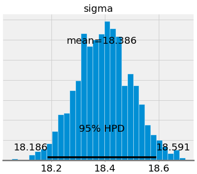
The first plots show the approximations of the posterior distributions of model parameters. These are the result of 1000 steps of MCMC, meaning the algorithm drew 1000 steps from the posterior distribution.
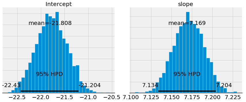
 If we compare the mean values for the slope and intercept to those obtained from OLS (the intercept from OLS was -21.83 and the slope was 7.17), we see that they are very similar. However, while we can use the mean as a single point estimate, we also have a range of possible values for the model parameters. As the number of data points increases, this range will shrink and converge one a single value representing greater confidence in the model parameters. (In Bayesian inference a range for a variable is called a credible interval and which has a slightly different interpretation from a confidence interval in frequentist inference).
When we want show the linear fit from a Bayesian model, instead of showing only estimate, we can draw a range of lines, with each one representing a different estimate of the model parameters. As the number of datapoints increases, the lines begin to overlap because there is less uncertainty in the model parameters.
In order to demonstrate the effect of the number of datapoints in the model, I used two models, the first, with the resulting fits shown on the left, used 500 datapoints and the one on the right used 15000 datapoints. Each graph shows 100 possible models drawn from the model parameter posteriors.
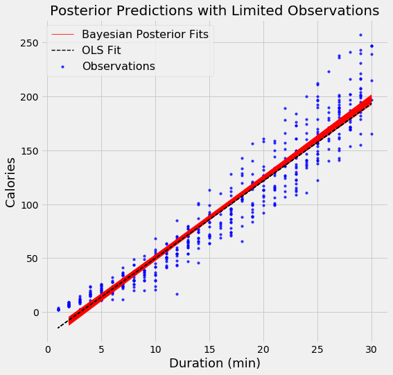
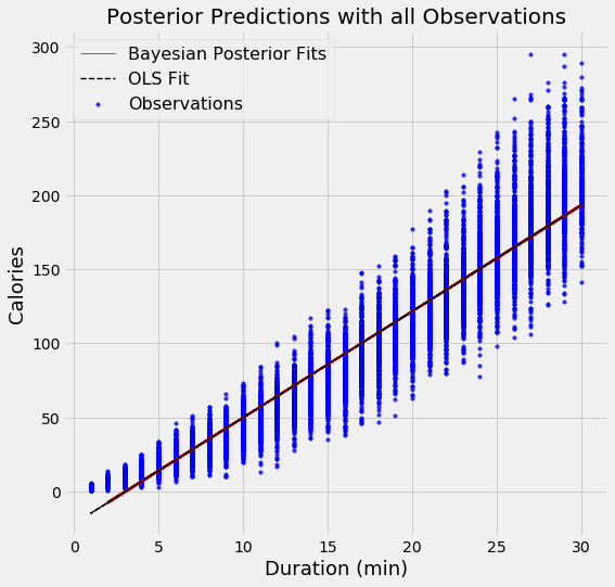 Bayesian Linear Regression Model Results with 500 (left) and 15000 observations (right)
There is much more variation in the fits when using fewer data points, which represents a greater uncertainty in the model. With all of the data points, the OLS and Bayesian Fits are nearly identical because the priors are washed out by the likelihoods from the data.
When predicting the output for a single datapoint using our Bayesian Linear Model, we also do not get a single value but a distribution. Following is the probability density plot for the number of calories burned exercising for 15.5 minutes. The red vertical line indicates the point estimate from OLS.
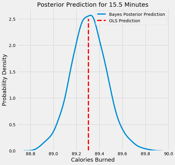 Posterior Probability Density of Calories Burned from Bayesian Model
We see that the probability of the number of calories burned peaks around 89.3, but the full estimate is a range of possible values.
Conclusions
Instead of taking sides in the Bayesian vs Frequentist debate (or any argument), it is more constructive to learn both approaches. That way, we can apply them in the right situation.
In problems where we have limited data or have some prior knowledge that we want to use in our model, the Bayesian Linear Regression approach can both incorporate prior information and show our uncertainty. Bayesian Linear Regression reflects the Bayesian framework: we form an initial estimate and improve our estimate as we gather more data. The Bayesian viewpoint is an intuitive way of looking at the world and Bayesian Inference can be a useful alternative to its frequentist counterpart. Data science is not about taking sides, but about figuring out the best tool for the job, and having more techniques in your repertoire only makes you more effective!
As always, I welcome feedback and constructive criticism. I can be reached on Twitter @koehrsen_will.
Sources