
Bayesian Linear Regression In Python Using Machine Learning To Predict Student Grades Part 2

Implementing a Model, Interpreting Results, and Making Predictions
In Part One of this Bayesian Machine Learning project, we outlined our problem, performed a full exploratory data analysis, selected our features, and established benchmarks. Here we will implement Bayesian Linear Regression in Python to build a model. After we have trained our model, we will interpret the model parameters and use the model to make predictions. The entire code for this project is available as a Jupyter Notebook on GitHub and I encourage anyone to check it out!
As a reminder, we are working on a supervised, regression machine learning problem. Using a dataset of student grades, we want to build a model that can predict a final student’s score from personal and academic characteristics of the student. The final dataset after feature selection is:
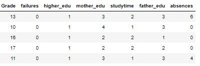
We have 6 features (explanatory variables) that we use to predict the target (response variable), in this case the grade. There are 474 students in the training set and 159 in the test set. To get a sense of the variable distributions (and because I really enjoy this plot) here is a Pairs plot of the variables showing scatter plots, histograms, density plots, and correlation coefficients.
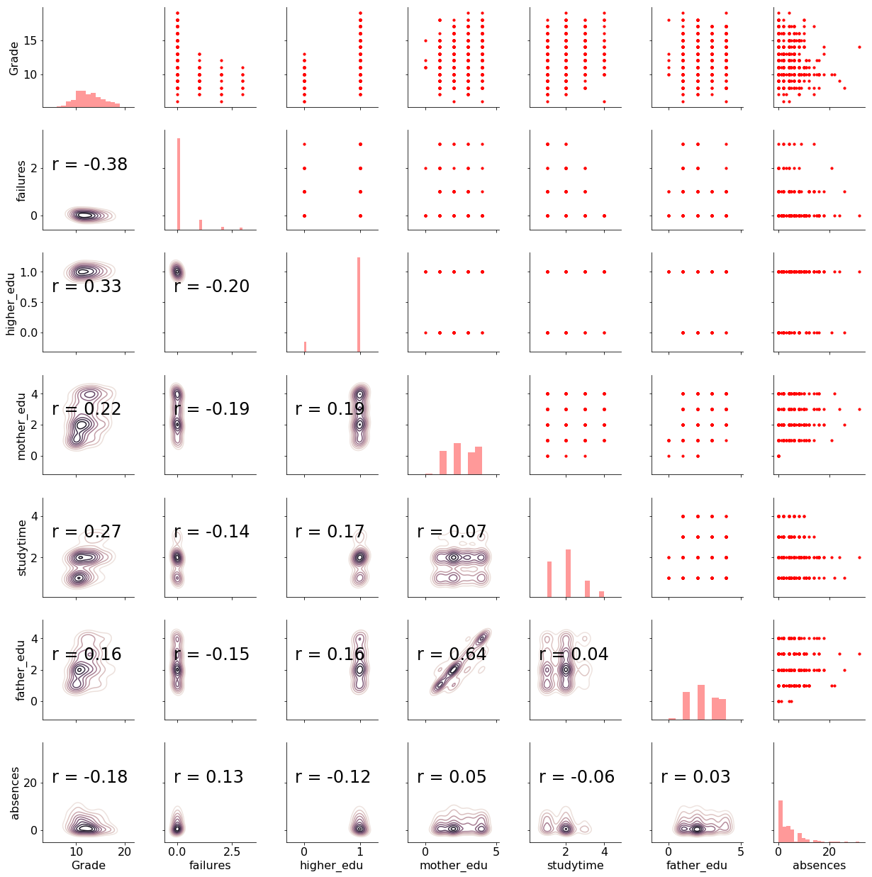
For details about this plot and the meaning of all the variables check out part one and the notebook. Now, let’s move on to implementing Bayesian Linear Regression in Python.
Bayesian Linear Regression
Let’s briefly recap Frequentist and Bayesian linear regression. The Frequentist view of linear regression assumes data is generated from the following model:
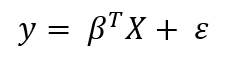 Where the response, y, is generated from the model parameters, β, times the input matrix, X, plus error due to random sampling noise or latent variables. In the ordinary least squares (OLS) method, the model parameters, β, are calculated by finding the parameters which minimize the sum of squared errors on the training data. The output from OLS is single point estimates for the “best” model parameters given the training data. These parameters can then be used to make predictions for new data points.
In contrast, Bayesian Linear Regression assumes the responses are sampled from a probability distribution such as the normal (Gaussian) distribution:
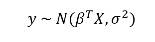 The mean of the Gaussian is the product of the parameters, β and the inputs, X, and the standard deviation is σ. In Bayesian Models, not only is the response assumed to be sampled from a distribution, but so are the parameters. The objective is to determine the posterior probability distribution for the model parameters given the inputs, X, and outputs, y:
![]() The posterior is equal to the likelihood of the data times the prior for the model parameters divided by a normalization constant. If we have some domain knowledge, we can use it to assign priors for the model parameters, or we can use non-informative priors: distributions with large standard deviations that do not assume anything about the variable. Using a non-informative prior means we “let the data speak.” A common prior choice is to use a normal distribution for β and a half-cauchy distribution for σ.
The posterior is equal to the likelihood of the data times the prior for the model parameters divided by a normalization constant. If we have some domain knowledge, we can use it to assign priors for the model parameters, or we can use non-informative priors: distributions with large standard deviations that do not assume anything about the variable. Using a non-informative prior means we “let the data speak.” A common prior choice is to use a normal distribution for β and a half-cauchy distribution for σ.
In practice, calculating the exact posterior distribution is computationally intractable for continuous values and so we turn to sampling methods such as Markov Chain Monte Carlo (MCMC) to draw samples from the posterior in order to approximate the posterior. Monte Carlo refers to the general technique of drawing random samples, and Markov Chain means the next sample drawn is based only on the previous sample value. The concept is that as we draw more samples, the approximation of the posterior will eventually converge on the true posterior distribution for the model parameters.
The end result of Bayesian Linear Modeling is not a single estimate for the model parameters, but a distribution that we can use to make inferences about new observations. This distribution allows us to demonstrate our uncertainty in the model and is one of the benefits of Bayesian Modeling methods. As the number of data points increases, the uncertainty should decrease, showing a higher level of certainty in our estimates.
Implementing Bayesian Linear Modeling in Python
The best library for probabilistic programming and Bayesian Inference in Python is currently PyMC3. It includes numerous utilities for constructing Bayesian Models and using MCMC methods to infer the model parameters. We will be using the Generalized Linear Models (GLM) module of PyMC3, in particular, the GLM.from_formula function which makes constructing Bayesian Linear Models extremely simple.
There are only two steps we need to do to perform Bayesian Linear Regression with this module:
- Build a formula relating the features to the target and decide on a prior distribution for the data likelihood
- Sample from the parameter posterior distribution using MCMC
Formula
Instead of having to define probability distributions for each of the model parameters separately, we pass in an R-style formula relating the features (input) to the target (output). Here is the formula relating the grade to the student characteristics:
**Grade ~ failures + higher_edu + mother_edu + studytime + father_edu + absences**
In this syntax, ~, is read as “is a function of”. We are telling the model that Grade is a linear combination of the six features on the right side of the tilde.
The model is built in a context using the with statement. In the call to GLM.from_formula we pass the formula, the data, and the data likelihood family (this actually is optional and defaults to a normal distribution). The function parses the formula, adds random variables for each feature (along with the standard deviation), adds the likelihood for the data, and initializes the parameters to a reasonable starting estimate. By default, the model parameters priors are modeled as a normal distribution.
Once the GLM model is built, we sample from the posterior using a MCMC algorithm. If we do not specify which method, PyMC3 will automatically choose the best for us. In the code below, I let PyMC3 choose the sampler and specify the number of samples, 2000, the number of chains, 2, and the number of tuning steps, 500.
In this case, PyMC3 chose the No-U-Turn Sampler and intialized the sampler with jitter+adapt_diag. To be honest, I don’t really know the full details of what these mean, but I assume someone much smarter than myself implemented them correctly. Sometimes just knowing how to use the tool is more important than understanding every detail of the implementation!
The sampler runs for a few minutes and our results are stored in normal_trace. This contains all the samples for every one of the model parameters (except the tuning samples which are discarded). The trace is essentially our model because it contains all the information we need to perform inference. To get an idea of what Bayesian Linear Regression does, we can examine the trace using built-in functions in PyMC3.
A traceplot shows the posterior distribution for the model parameters on the left and the progression of the samples drawn in the trace for the variable on the right. The two colors represent the two difference chains sampled.
pm.traceplot(normal_trace)
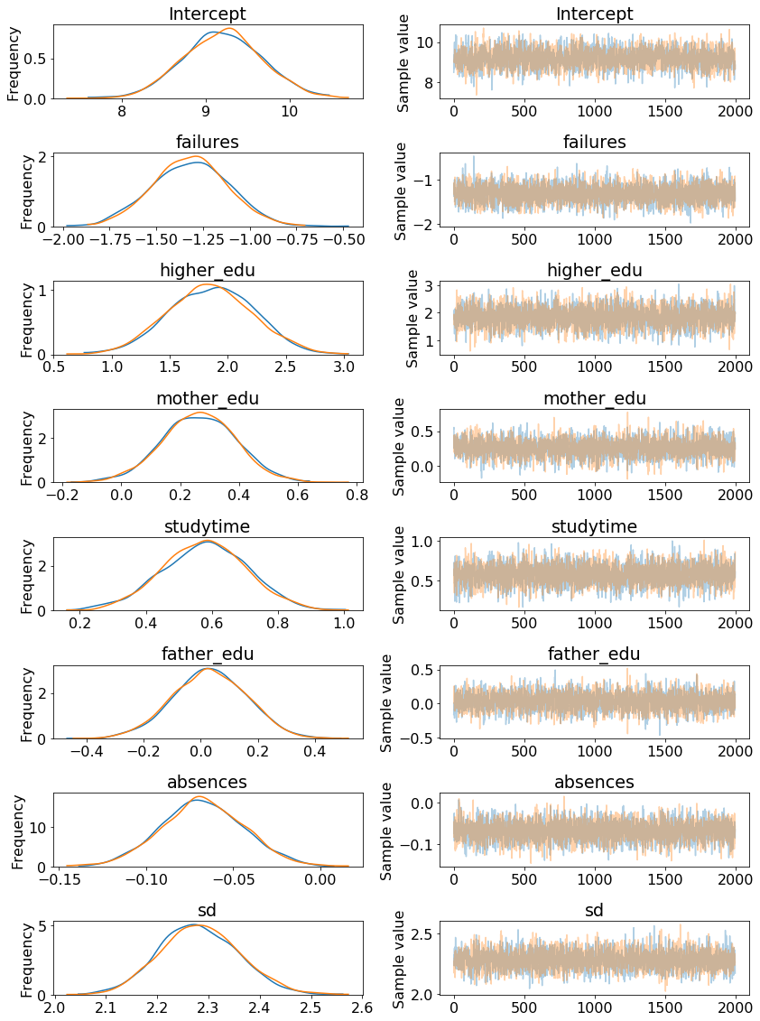 Here we can see that our model parameters are not point estimates but distributions. The mean of each distribution can be taken as the most likely estimate, but we also use the entire range of values to show we are uncertain about the true values.
Another way to look at the posterior distributions is as histograms:
pm.plot_posterior(normal_trace)
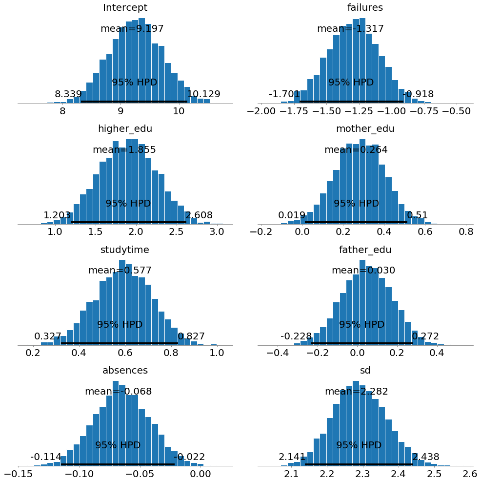 Here we can see the mean, which we can use as most likely estimate, and also the entire distribution. 95% HPD stands for the 95% Highest Posterior Density and is a credible interval for our parameters. A credible interval is the Bayesian equivalent of a confidence interval in Frequentist statistics (although with different interpretations).
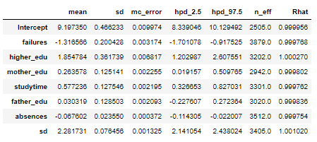
We can also see a summary of all the model parameters:
pm.df_summary(normal_trace)
 We can interpret these weights in much the same way as those of OLS linear regression. For example in the model:
- Previous class failures and absences have a negative weight
- Higher Education plans and studying time have a positive weight
- The mother’s and father’s education have a positive weight (although the mother’s is much more positive)
The standard deviation column and hpd limits give us a sense of how confident we are in the model parameters. For example, the father_edu feature has a 95% hpd that goes from -0.22 to 0.27 meaning that we are not entirely sure if the effect in the model is either negative or positive! There is also a large standard deviation (the sd row) for the data likelihood, indicating large uncertainty in the targets. Overall, we see considerable uncertainty in the model because we are dealing with a small number of samples. With only several hundred students, we do not have enough data to pin down the model parameters precisely.
Interpret Variable Effects
In order to see the effect of a single variable on the grade, we can change the value of this variable while holding the others constant and look at how the estimated grades change. To do this, we use the plot_posterior_predictive function and assume that all variables except for the one of interest (the query variable) are at the median value. We generate a range of values for the query variable and the function estimates the grade across this range by drawing model parameters from the posterior distribution. Here’s the code:
The results show the estimated grade versus the range of the query variable for 100 samples from the posterior:
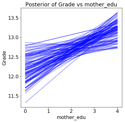
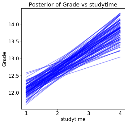
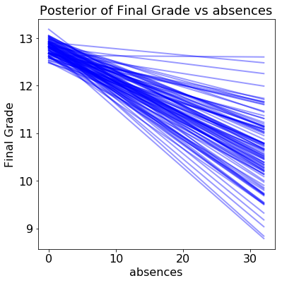 Each line (there are 100 in each plot) is drawn by picking one set of model parameters from the posterior trace and evaluating the predicted grade across a range of the query variable. The distribution of the lines shows uncertainty in the model parameters: the more spread out the lines, the less sure the model is about the effect of that variable.
For one variable, the father’s education, our model is not even sure if the effect of increasing the variable is positive or negative!
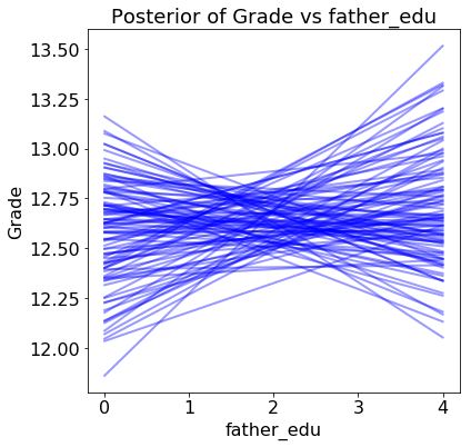 If we were using this model to make decisions, we might want to think twice about deploying it without first gathering more data to form more certain estimates. With only several hundred students, there is considerable uncertainty in the model parameters. For example, we should not make claims such as “the father’s level of education positively impacts the grade” because the results show there is little certainly about this conclusion.
If we were using Frequentist methods and saw only a point estimate, we might make faulty decisions because of the limited amount of data. In cases where we have a limited dataset, Bayesian models are a great choice for showing our uncertainty in the model.
Making Predictions
When it comes to predicting, the Bayesian model can be used to estimate distributions. We remember that the model for Bayesian Linear Regression is:
Where β is the coefficient matrix (model parameters), X is the data matrix, and σ is the standard deviation. If we want to make a prediction for a new data point, we can find a normal distribution of estimated outputs by multiplying the model parameters by our data point to find the mean and using the standard deviation from the model parameters.
In this case, we will take the mean of each model parameter from the trace to serve as the best estimate of the parameter. If we take the mean of the parameters in the trace, then the distribution for a prediction becomes:
**Grade ~ N(9.20 * Intercept - 1.32 * failures + 1.85 * higher_edu + 0.26 * mother_edu + 0.58 * studytime + 0.03 * father_edu - 0.07 * absences, 2.28^2)**
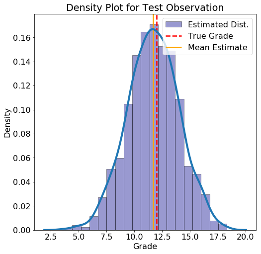
For a new data point, we substitute in the value of the variables and construct the probability density function for the grade. As an example, here is an observation from the test set along with the probability density function (see the Notebook for the code to build this distribution):
**Test Observation:
failures = 0, higher_edu = 1, mother_edu = 2, studytime = 1,
father_edu = 2, absences = 8**
 ```
```
True Grade = 12 Average Estimate = 11.6763 5% Estimate = 7.7618 95% Estimate = 15.5931
For this data point, the mean estimate lines up well with the actual grade, but there is also a wide estimated interval. If we had more students, the uncertainty in the estimates should be lower.

We can also make predictions for any new point that is not in the test set:
New Observation: absences = 1, failures = 0, father_edu = 1 higher_edu = 1, mother_edu = 4, studytime = 3
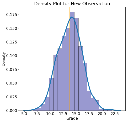
*```*
**Average Estimate = 13.8009
5% Estimate = 10.0696 95% Estimate = 17.4629**
Comparison to Standard Machine Learning Models
In the first part of this series, we calculated benchmarks for a number of standard machine learning models as well as a naive baseline. To calculate the MAE and RMSE metrics, we need to make a single point estimate for all the data points in the test set. We can make a “most likely” prediction using the means value from the estimated distributed. The resulting metrics, along with those of the benchmarks, are shown below:
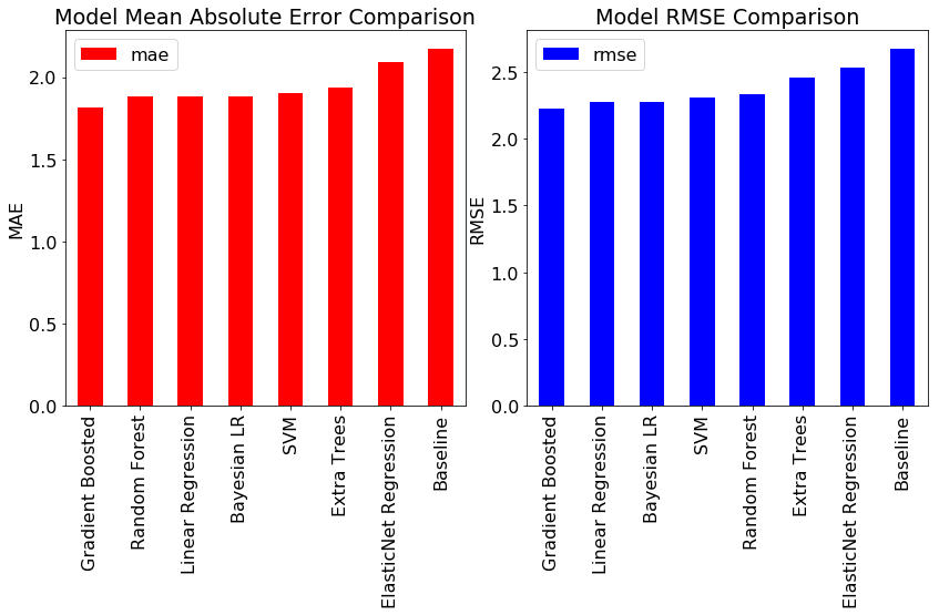 Bayesian Linear Regression achieves nearly the same performance as the best standard models! However, the main benefits of Bayesian Linear Modeling are not in the accuracy, but in the interpretability and the quantification of our uncertainty. Any model is only an estimate of the real world, and here we have seen how little confidence we should have in models trained on limited data.
Next Steps
For anyone looking to get started with Bayesian Modeling, I recommend checking out the notebook. In this project, I only explored half of the student data (I used math scores and the other half contains Portuguese class scores) so feel free to carry out the same analysis on the other half. In addition, we can change the distribution for the data likelihood—for example to a Student’s T distribution — and see how that changes the model. As with most machine learning, there is a considerable amount that can be learned just by experimenting with different settings and often no single right answer!
Conclusions
In this series of articles, we walked through the complete machine learning process used to solve a data science problem. We started with exploratory data analysis, moved to establishing a baseline, tried out several different models, implemented our model of choice, interpreted the results, and used the model to make new predictions. While the model implementation details may change, this general structure will serve you well for most data science projects. Moreover, hopefully this project has given you an idea of the unique capabilities of Bayesian Machine Learning and has added another tool to your skillset. Learning new skills is the most exciting aspect of data science and now you have one more to deploy to solve your data problems.
As always, I welcome feedback and constructive criticism. I can be reached on Twitter @koehrsen_will.