A Complete Real-World Implementation

The past few months, I encountered one term again and again in the data science world: Markov Chain Monte Carlo. In my research lab, in podcasts, in articles, every time I heard the phrase I would nod and think that sounds pretty cool with only a vague idea of what anyone was talking about. Several times I tried to learn MCMC and Bayesian inference, but every time I started reading the books, I soon gave up. Exasperated, I turned to the best method to learn any new skill: apply it to a problem.

Using some of my sleep data I had been meaning to explore and a hands-on application-based book (Bayesian Methods for Hackers, available free online), I finally learned Markov Chain Monte Carlo through a real-world project. As usual, it was much easier (and more enjoyable) to understand the technical concepts when I applied them to a problem rather than reading them as abstract ideas on a page. This article walks through the introductory implementation of Markov Chain Monte Carlo in Python that finally taught me this powerful modeling and analysis tool.

The full code and data for this project is on GitHub. I encourage anyone to take a look and use it on their own data. This article focuses on applications and results, so there are a lot of topics covered at a high level, but I have tried to provide links for those wanting to learn more!

Introduction

My Garmin Vivosmart watch tracks when I fall asleep and wake up based on heart rate and motion. It’s not 100% accurate, but real-world data is never perfect, and we can still extract useful knowledge from noisy data with the right model!

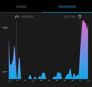Typical Sleep Data

The objective of this project was to use the sleep data to create a model that specifies the posterior probability of sleep as a function of time. As time is a continuous variable, specifying the entire posterior distribution is intractable, and we turn to methods to approximate a distribution, such as Markov Chain Monte Carlo (MCMC).

Choosing a Probability Distribution

Before we can start with MCMC, we need to determine an appropriate function for modeling the posterior probability distribution of sleep. One simple way to do this is to visually inspect the data. The observations for when I fall asleep as a function of time are shown below.

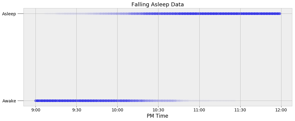Sleeping Data

Every data point is represented as a dot, with the intensity of the dot showing the number of observations at the specific time. My watch records only the minute at which I fall asleep, so to expand the data, I added points to every minute on both sides of the precise time. If my watch says I fell asleep at 10:05 PM, then every minute before is represented as a 0 (awake) and every minute after gets a 1 (asleep). This expanded the roughly 60 nights of observations into 11340 data points.

We can see that I tend to fall asleep a little after 10:00 PM but we want to create a model that captures the transition from awake to asleep in terms of a probability. We could use a simple step function for our model that changes from awake (0) to asleep (1) at one precise time, but this would not represent the uncertainty in the data. I do not go to sleep at the same time every night, and we need a function to that models the transition as a gradual process to show the variability. The best choice given the data is a logistic function which is smoothly transitions between the bounds of 0 and 1. Following is a logistic equation for the probability of sleep as a function of time

Here, β (beta) and α (alpha) are the parameters of the model that we must learn during MCMC. A logistic function with varying parameters is shown below.

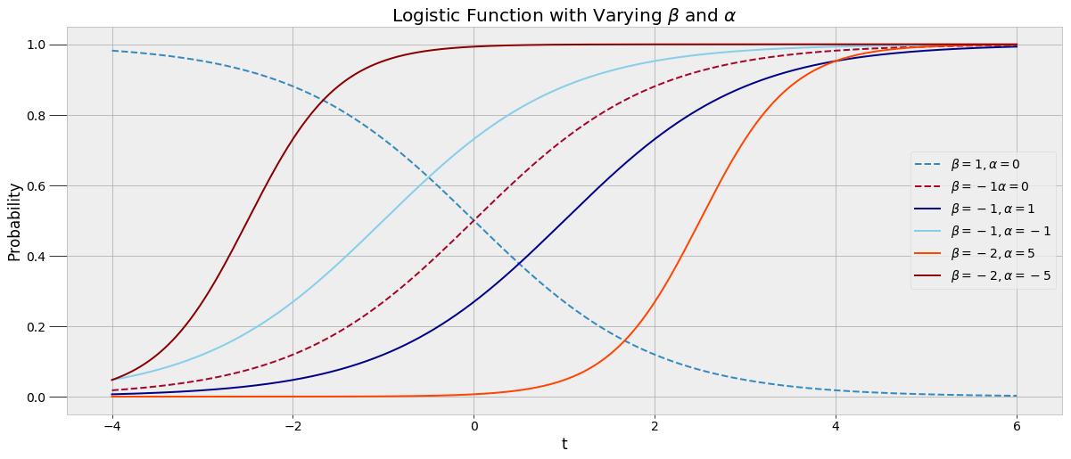A logistic function fits the data because the probability of being asleep transitions gradually, capturing the variability in my sleep patterns. We want to be able to plug in a time t to the function and get out the probability of sleep, which must be between 0 and 1. Rather than a straight yes or no answer to the question am I asleep at 10:00 PM, we can get a _probability._ To create this model, we use the data to find the best alpha and beta parameters through one of the techniques classified as Markov Chain Monte Carlo.

Markov Chain Monte Carlo

Markov Chain Monte Carlo refers to a class of methods for sampling from a probability distribution in order to construct the most likely distribution. We cannot directly calculate the logistic distribution, so instead we generate thousands of values — called samples — for the parameters of the function (alpha and beta) to create an approximation of the distribution. The idea behind MCMC is that as we generate more samples, our approximation gets closer and closer to the actual true distribution.

There are two parts to a Markov Chain Monte Carlo method. Monte Carlo refers to a general technique of using repeated random samples to obtain a numerical answer. Monte Carlo can be thought of as carrying out many experiments, each time changing the variables in a model and observing the response. By choosing random values, we can explore a large portion of the parameter space, the range of possible values for the variables. A parameter space for our problem using normal priors for the variables (more on this in a moment) is shown below.

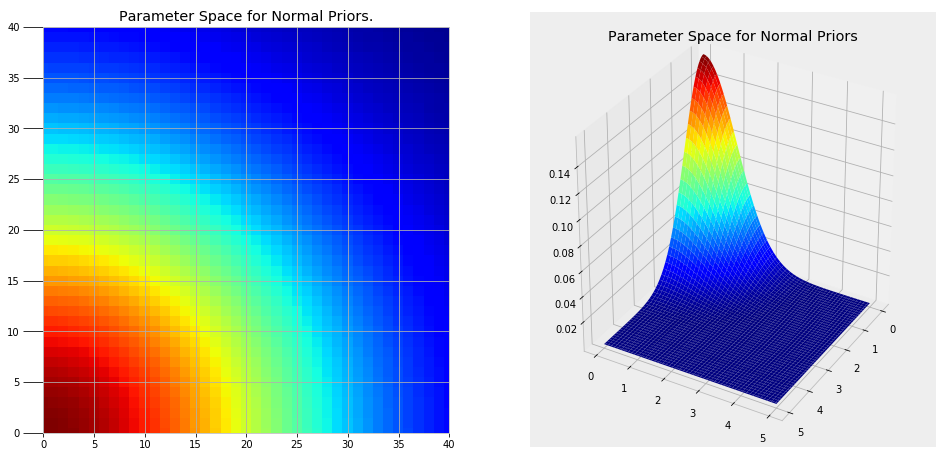Clearly we cannot try every single point in these plots, but by randomly sampling from regions of higher probability (red) we can create the most likely model for our problem.

Markov Chain

A Markov Chain is a process where the next state depends only on the current state. (A state in this context refers to the assignment of values to the parameters). A Markov Chain is memoryless because only the current state matters and not how it arrived in that state. If that’s a little difficult to understand, consider an everyday phenomenon, the weather. If we want to predict the weather tomorrow we can get a reasonable estimate using only the weather today. If it snowed today, we look at historical data showing the distribution of weather on the day after it snows to estimate probabilities of the weather tomorrow. The concept of a Markov Chain is that we do not need to know the entire history of a process to predict the next output, an approximation that works well in many real-world situations.

Putting together the ideas of Markov Chain and Monte Carlo, MCMC is a method that repeatedly draws random values for the parameters of a distribution based on the current values. Each sample of values is random, but the choices for the values are limited by the current state and the assumed prior distribution of the parameters. MCMC can be considered as a random walk that gradually converges to the true distribution.

In order to draw random values of alpha and beta, we need to assume a prior distribution for these values. As we have no assumptions about the parameters ahead of time, we can use a normal distribution. The normal, or Gaussian distribution, is defined by the mean, showing the location of the data, and the variance, showing the spread. Several normal distributions with different means and spreads are below:

The specific MCMC algorithm we are using is called Metropolis Hastings. In order to connect our observed data to the model, every time a set of random values are drawn, the algorithm evaluates them against the data. If they do not agree with the data (I’m simplifying a little here), the values are rejected and the model remains in the current state. If the random values are in agreement with the data, the values are assigned to the parameters and become the current state. This process continues for a specified number of steps, with the accuracy of the model improving with the number of steps.

Putting it all together, the basic procedure for Markov Chain Monte Carlo in our problem is as follows:

1. Select an initial set of values for alpha and beta, the parameters of the logistic function.
2. Randomly assign new values to alpha and beta based on the current state.
3. Check if the new random values agree with the observations. If they do not, reject the values and return to the previous state. If they do, accept the values as the new current state.
4. Repeat steps 2 and 3 for the specified number of iterations.

The algorithm returns all of the values it generates for alpha and beta. We can then use the average of these values as the most likely final values for alpha and beta in the logistic function. MCMC cannot return the “True” value but rather an approximation for the distribution. The final model for the probability of sleep given the data will be the logistic function with the average values of alpha and beta.

Python Implementation

The above details went over my head many times until I applied them in Python! Seeing the results first-hand is a lot more helpful than reading someone else describe. To implement MCMC in Python, we will use the PyMC3 Bayesian inference library. It abstracts away most of the details, allowing us to create models without getting lost in the theory.

The following code creates the full model with the parameters, alpha and beta, the probability, p, and the observations, observed The step variable refers to the specific algorithm, and the sleep_trace holds all of the values of the parameters generated by the model.

(Check out the notebook for the full code)

To get a sense of what occurs when we run this code, we can look at all the value of alpha and beta generated during the model run.

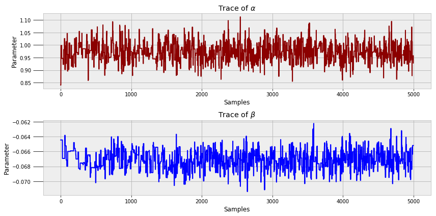These are called trace plots. We can see that each state is correlated to the previous — the Markov Chain — but the values oscillate significantly — the Monte Carlo sampling.

In MCMC, it is common practice to discard up to 90% of the trace. The algorithm does not immediately converge to the true distribution and the initial values are often inaccurate. The later values for the parameters are generally better which means they are what we should use for building our model. We used 10000 samples and discarded the first 50%, but an industry application would likely use hundreds of thousands or millions of samples.

MCMC converges to the true value given enough steps, but assessing convergence can be difficult. I will leave that topic out of this post (one way is by measuring the auto-correlation of the traces) but it is an important consideration if we want the most accurate results. PyMC3 has built in functions for assessing the quality of models, including trace and autocorrelation plots.

pm.traceplot(sleep_trace, ['alpha', 'beta'])
pm.autocorrplot(sleep_trace, ['alpha', 'beta'])

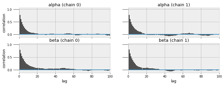Trace (left) and autocorrelation (right) plots

Sleep Model

After finally building and running the model, it’s time to use the results. We will the the average of the last 5000 alpha and beta samples as the most likely values for the parameters which allows us to create a single curve modeling the posterior sleep probability:

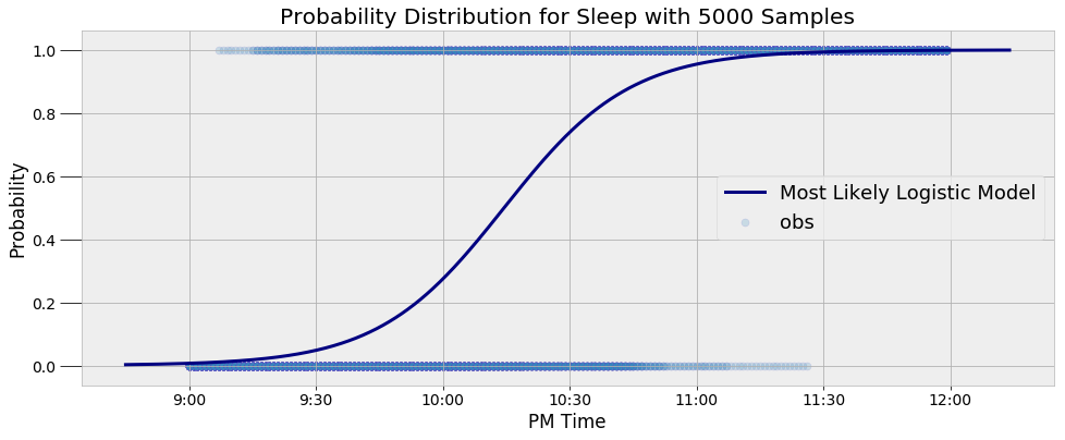The model represents the data well. Moreover, it captures the inherent variability in my sleep patterns. Rather than a single yes or no answer, the model gives us a probability. For example, we can query the model to find out the probability I am asleep at a given time and find the time at which the probability of being asleep passes 50%:

**9:30  PM probability of being asleep: 4.80%.
10:00 PM probability of being asleep: 27.44%.
10:30 PM probability of being asleep: 73.91%.**

**The probability of sleep increases to above 50% at 10:14 PM.**

Although I try to go to bed at 10:00 PM, that clearly does not happen most nights! We can see that the average time I go to bed is around 10:14 PM.

These values are the most likely estimates given the data. However, there is uncertainty associated with these probabilities because the model is approximate. To represent this uncertainty, we can make predictions of the sleep probability at a given time using all of the alpha and beta samples instead of the average and then plot a histogram of the results.

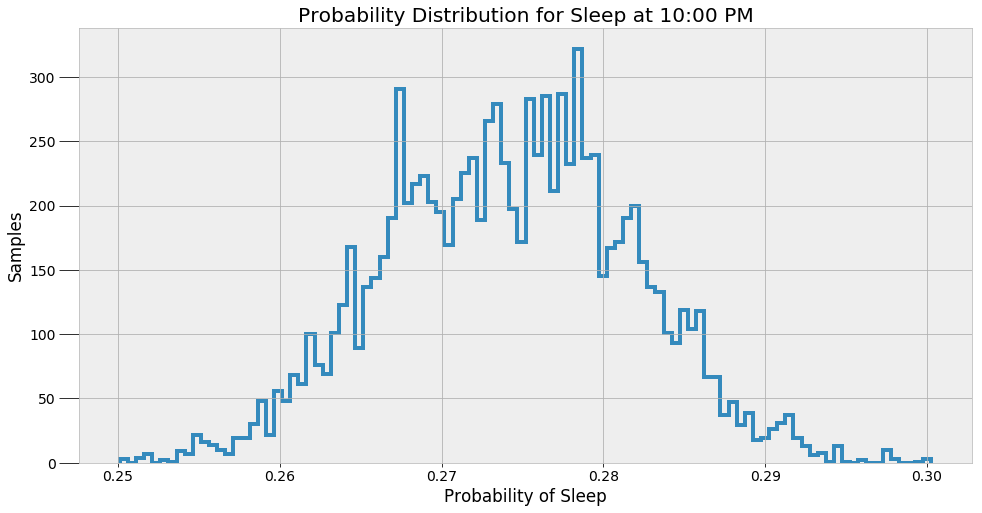
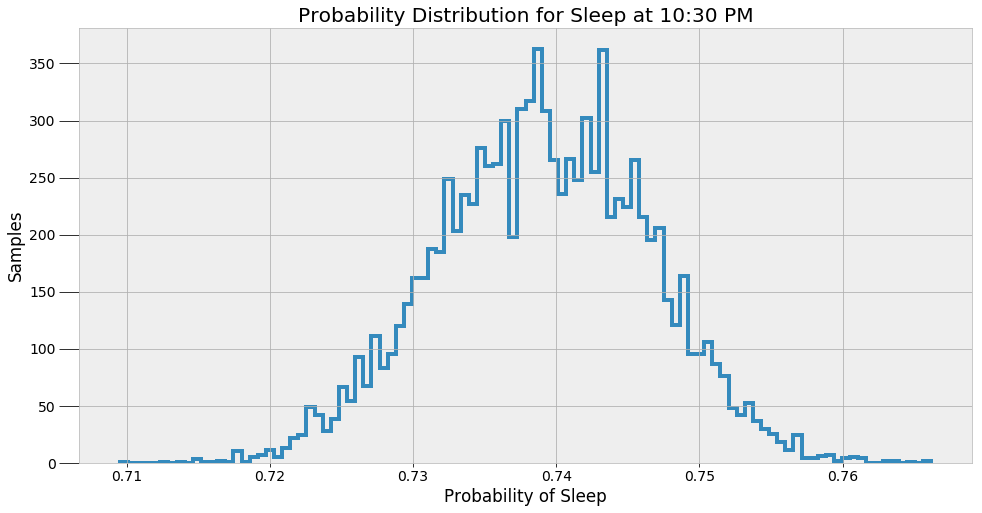These results give a better indicator of what an MCMC model really does. The method does not find a single answer, but rather a sample of possible values. Bayesian Inference is useful in the real-world because it expresses predictions in terms of probabilities. We can say there is one most likely answer, but the more accurate response is that there are a range of values for any prediction.

Wake Model

I can use the waking data to find a similar model for when I wake up in the morning. I try to always be up at 6:00 AM with my alarm, but we can see that does not always happen! The following image shows the final model for the transition from sleeping to waking along with the observations.

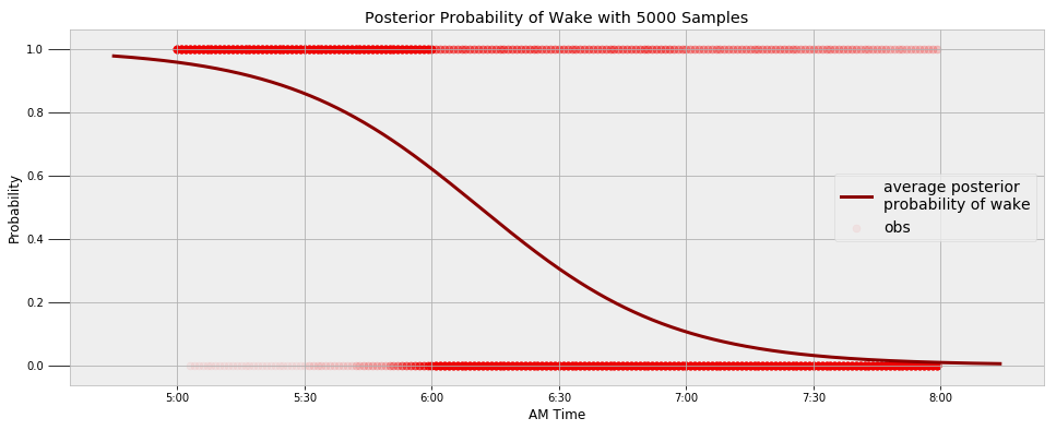We can query the model to find the probability I’m asleep at a given time and the most likely time for me to wake up.

**Probability of being awake at 5:30 AM: 14.10%.
Probability of being awake at 6:00 AM: 37.94%.
Probability of being awake at 6:30 AM: 69.49%.**

**The probability of being awake passes 50% at 6:11 AM.**

Looks like I have some work to do with that alarm!

Duration of Sleep

A final model I wanted to create — both out of curiosity and for the practice — was my duration of sleep. First, we need to find a function to model the distribution of the data. Ahead of time, I think it would be normal, but we can only find out by examining the data!

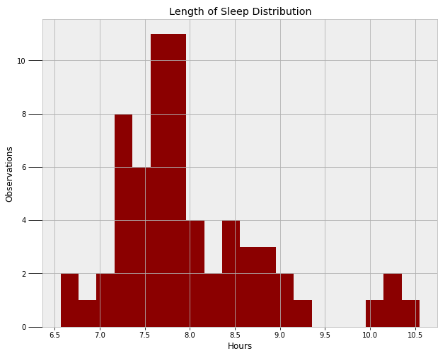A normal distribution would work, but it would not capture the outlying points on the right side (times when I severely slept in). We could use two separate normal distributions to represent the two modes, but instead, I will use a skewed normal. The skewed normal has three parameters, the mean, the variance, and alpha, the skew. All three of these must be learned from the MCMC algorithm. The following code creates the model and implements the Metropolis Hastings sampling.

Now, we can use the average values of the three parameters to construct the most likely distribution. Following is the final skewed normal distribution on top of the data.

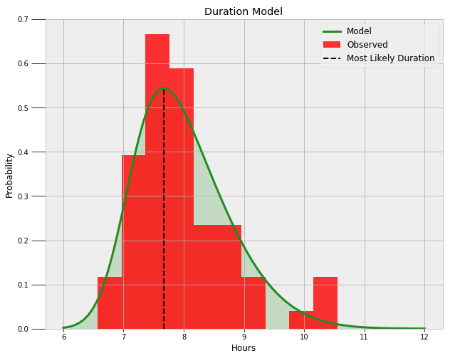It looks like a nice fit! We can query the model to find the likelihood I get at least a certain amount of sleep and the most likely duration of sleep:

**Probability of at least 6.5 hours of sleep = 99.16%.
Probability of at least 8.0 hours of sleep = 44.53%.
Probability of at least 9.0 hours of sleep = 10.94%.**

**The most likely duration of sleep is 7.67 hours.**

I’m not entirely pleased with those results, but what can you expect as a graduate student?

Conclusions

Once again, completing this project showed me the importance of solving problems, preferably ones with real world applications! Along the way to building an end-to-end implementation of Bayesian Inference using Markov Chain Monte Carlo, I picked up many of the fundamentals and enjoyed myself in the process. Not only did I learn a little bit about my habits (and what I need to improve), but now I can finally understand what everyone is talking about when they say MCMC and Bayesian Inference. Data science is about constantly adding tools to your repertoire and the most effective way to do that is to find a problem and get started!

As always, I welcome feedback and constructive criticism. I can be reached on Twitter @koehrsen_will.