Using Bayesian Inference on a real-world problem

The fundamental idea of Bayesian inference is to become “less wrong” with more data. The process is straightforward: we have an initial belief, known as a prior, which we update as we gain additional information. Although we don’t think about it as Bayesian Inference, we use this technique all the time. For example, we might initially think there is a 50% chance we will get a promotion at the end of the quarter. If we receive positive feedback from our manager, we adjust our estimate upwards, and conversely, we might decrease the probability if we make a mess with the coffee machine. As we continually gather information, we refine our estimate to get closer to the “true” answer.

Our intuitive actions are formalized in the simple yet powerful equation known as Bayes’ Rule:

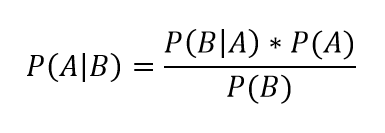
We read the left side, called the posterior, as the conditional probability of event A given event B. On the right side, P(A) is our prior, or the initial belief of the probability of event A, P(B|A) is the likelihood (also a conditional probability), which we derive from our data, and P(B) is a normalization constant to make the probability distribution sum to 1. The general form of Bayes’ Rule in statistical language is the posterior probability equals the likelihood times the prior divided by the normalization constant. This short equation leads to the entire field of Bayesian Inference, an effective method for reasoning about the world.

While A’s and B’s may be good placeholders, they aren’t very helpful for letting us see how we can use this concept. To do that, we can apply Bayes’ Rule to a problem with real world data.

One problem I have been exploring in my own life is sleeping patterns. I have more than 2 months of data from my Garmin Vivosmart watch showing when I fall asleep and wake up. In a previous post, I figured out the probability I am asleep at a given time using Markov Chain Monte Carlo (MCMC) methods.The final model showing the most likely distribution of sleep as a function of time (MCMC is an approximate method) is below.

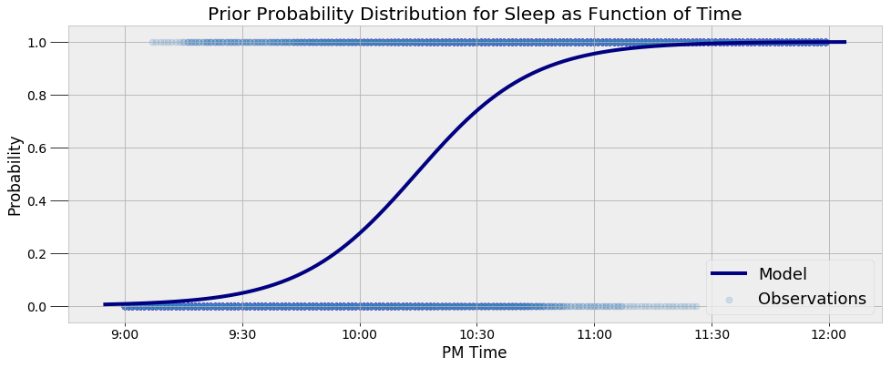This is the probability I am asleep taking into account only the time. What if we know the time and have additional evidence? How would knowing that my bedroom light is on change the probability that I am asleep? This is where we use Bayes’ Rule to update our estimate. For a specific time, if we know information about my bedroom light, we can use the probability from the distribution above as the _prior_ and then apply Bayes’ equation:

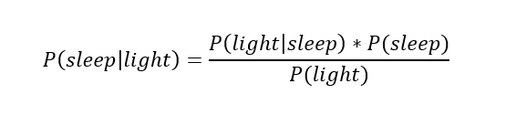The left side is the posterior, the conditional probability of sleep given the status of my bedroom light (either on or off). The probability at a given time will serve as our prior, P(sleep) , or the estimate we use if we have no additional information. For example, at 10:00 PM, the prior probability I am asleep is 27.34%. If we do have more information, we can update this using the likelihood, P(bedroom light |sleep) , which is derived from observed data. Based on my habits, I know the probability my bedroom light is on given that I am asleep is about 1%. That is:

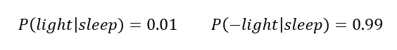The probability that my light is _off_ given I am asleep is 1–0.01 = 0.99(Here I am using the minus sign (-) to indicate the opposite condition.) This is because conditional probability distributions must sum to 1. If we know I am asleep, either my bedroom light has to be on or it has to be off!

The final piece of the equation is the normalization constant P(light) . This represents the total probability my light is on. There are two conditions for which my light is on: I am asleep or I am awake. Therefore, if we know the prior probability of sleep, we can calculate the normalization constant as:

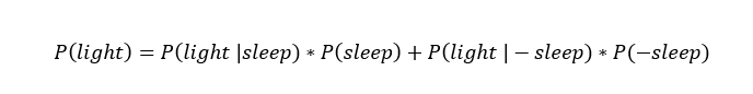The total probability my light is on takes into account both the chance I am asleep and my light is on and the chance I am awake and my light is on. (P(-sleep) = 1 — P(sleep) is the probability I am awake.)

The probability my light is on given that I am not asleep, P(light | — sleep), is also determined from observations. In my case, I know there is around a 80% probability my bedroom light is on if I am awake (which means there is a 20% chance my light is not on if I’m awake).

Using the total probability for my light being on, Bayes’ equation is:

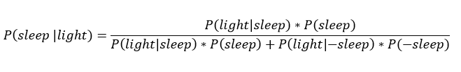This represents the probability I am asleep given that my light is on. If my light is off, then we replace every P(light|... with P(-light|....

That’s more than enough equations with only words, let’s see how we can use this with numbers!

We will walk through applying the equation for a time of 10:30 PM if we know my light is on. First, we calculate the prior probability I am asleep using the time and get an answer of 73.90%. The prior provides a good starting point for our estimate, but we can improve it by incorporating info about my light. Knowing that my light is on, we can fill in Bayes’ Equation with the relevant numbers:

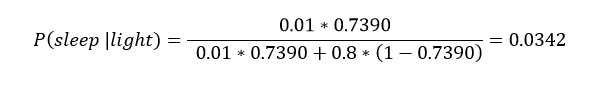The knowledge that my light is on drastically changes our estimate of the probability I am asleep from over 70% to 3.42%. This shows the power of Bayes’ Rule: we were able to update our initial estimate for the situation by incorporating more information. While we might have intuitively done this anyway, thinking about it in terms of formal equations allows us to update our beliefs in a rigorous manner.

Let’s try another example. What if it is 9:45 PM, and my light is off? Try to work this one out starting with the prior probability of 0.1206.

Instead of always doing this inference by hand, I wrote some simple Python code to do these calculations which you can play with in the Jupyter Notebook. The code outputs the following answer:

Time: 09:45:00 PM 	Light is OFF.

The prior probability of sleep:    12.06%
The updated probability of sleep:  40.44%

We again see the extra information changes our estimate. Now, if my sister wants to call me at 9:45 PM and she somehow knows that my light is on, she can consult this equation to determine if I will pick up (assuming I always pick up when I’m awake)! Who says you can’t use stats in your daily life?

Seeing the numerical results is helpful, but visualizations can also be useful for making the point clearer. I always try to incorporate plots to communicate ideas if they don’t come across just by looking at equations. Here, we can visualize the prior and the conditional probability distribution of sleep using the extra data.

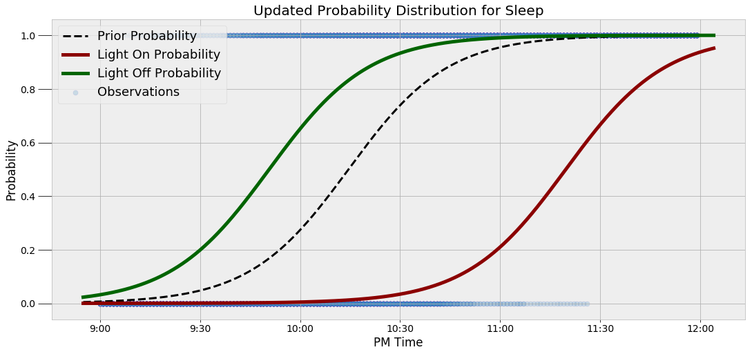When my light is on, the curve is shifted to the right, indicating there is a lower probability I am asleep at a given time. Likewise, the curve is shifted to the left if my light is off. It can be difficult to conceptually understand a statistical concept, but this illustration demonstrates precisely why we use Bayes’ Rule. If we want to be less wrong about the world, then additional information should change our beliefs, and Bayesian Inference updates our estimates using a systematic method.

Using More Evidence!

Why stop with my bedroom light? We can use as much information in the model as we like and it will continue to get more precise (as long as the data tells us something useful about the situation). For example, if I know the likelihood my phone is charging given that I am asleep is 95%, we can incorporate that knowledge into the model.

Here, we will assume the probability my phone is charging is conditionally independent of the probability my light is on given the information of whether or not I am sleeping (independence is a little more advanced concept, but it allows us to simplify many problems). Bayes’ equation using the extra information is expressed:

That might look intimidating, but using a little Python code, we can make a function to do the calculation for us. We feed in any time, and any combination of whether or not my light is on and phone is charging and the function returns the updated probability I am asleep.

I’ll skip the math (I let my computer do it anyway) and show the results:

Time is 11:00:00 PM 	Light is ON 	Phone IS NOT charging.

The prior probability of sleep:    95.52%
The updated probability of sleep:  1.74%

At 11:00 PM, with no additional information, we would guess with almost certainty that I am asleep. However, once we have the additional information that my light is on and phone is not charging, we conclude there is only a miniscule chance I am asleep. Here’s another query:

Time is 10:15:00 PM 	Light is OFF 	Phone IS charging.

The prior probability of sleep:    50.79%
The updated probability of sleep:  95.10%

The probability shifts lower or higher depending on the exact situation. To demonstrate this, we can look at the four configurations of light and phone evidence and how they change the probability distribution:

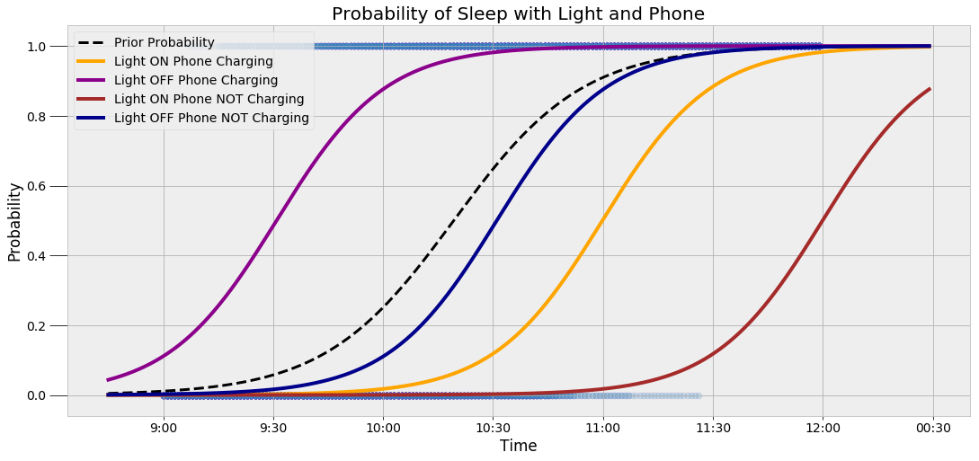There is a lot of information in this graph, but the critical idea is that the probability curve changes depending on the evidence. As we get more data, we can further refine our estimate.

Conclusion

Bayes’ Rule and other statistical concepts can be difficult to understand when presented with abstract equations using only letters or made-up situations. I’ve been through many classes where Bayes Rule was shown in terms of not very useful examples like coin flips or drawing colored balls from an urn, but it wasn’t until this project that I finally understood the applicability of Bayesian inference. If you’re struggling with a concept, seek out a situation where you can apply it, or look at cases where others have already done so!

Actual learning comes when we translate concepts to problems. Not only can we learn new skills this way, but we can also do some pretty cool projects! Success in data science is about continuously learning, adding new techniques to your skillset, and figuring out the best method for different tasks. Here we showed how Bayesian Inference lets us update our beliefs to account for new evidence in order to better model reality. We constantly need to adjust our predictions as we gather more evidence, and Bayes’ Equation provides us with the appropriate framework.

As always, I welcome feedback, discussion, and constructive criticism. I can be reached on Twitter @koehrsen_will.