(Source)

Using the Gradient Boosting Regressor to show uncertainty in machine learning estimates

“All models are wrong but some are useful” — George Box. It’s critical to keep this sage advice in mind when we present machine learning predictions. With all machine learning pipelines, there are limitations: features which affect the target that are not in the data (latent variables), or assumptions made by the model which don’t align with reality. These are overlooked when we show a single exact number for a prediction — the house will be $450,300.01 —which gives the impression we are entirely confident our model is a source of truth.

A more honest way to show predictions from a model is as a range of estimates: there might be a most likely value, but there is also a wide interval where the real value could be. This isn’t a topic typically addressed in data science courses, but it’s crucial that we show uncertainty in predictions and don’t oversell the capabilities of machine learning. While people crave certainty, I think it’s better to show a wide prediction interval that does contain the true value than an exact estimate which is far from reality.

In this article, we’ll walk through one method of producing uncertainty intervals in Scikit-Learn. The full code is available on GitHub with an interactive version of the Jupyter Notebook on nbviewer. We’ll focus primarily on implementation, with a brief section and resources for understanding the theory at the end. Generating prediction intervals is another tool in the data science toolbox, one critical for earning the trust of non-data-scientists.

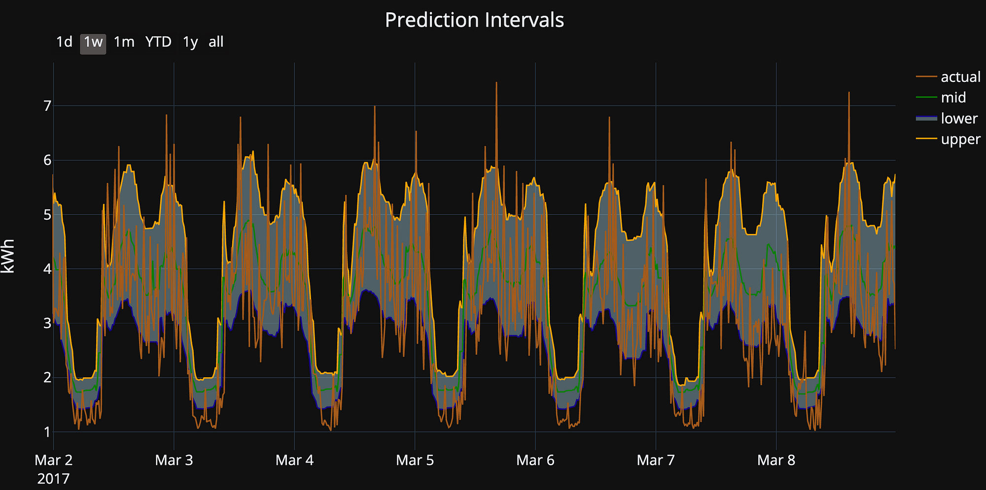
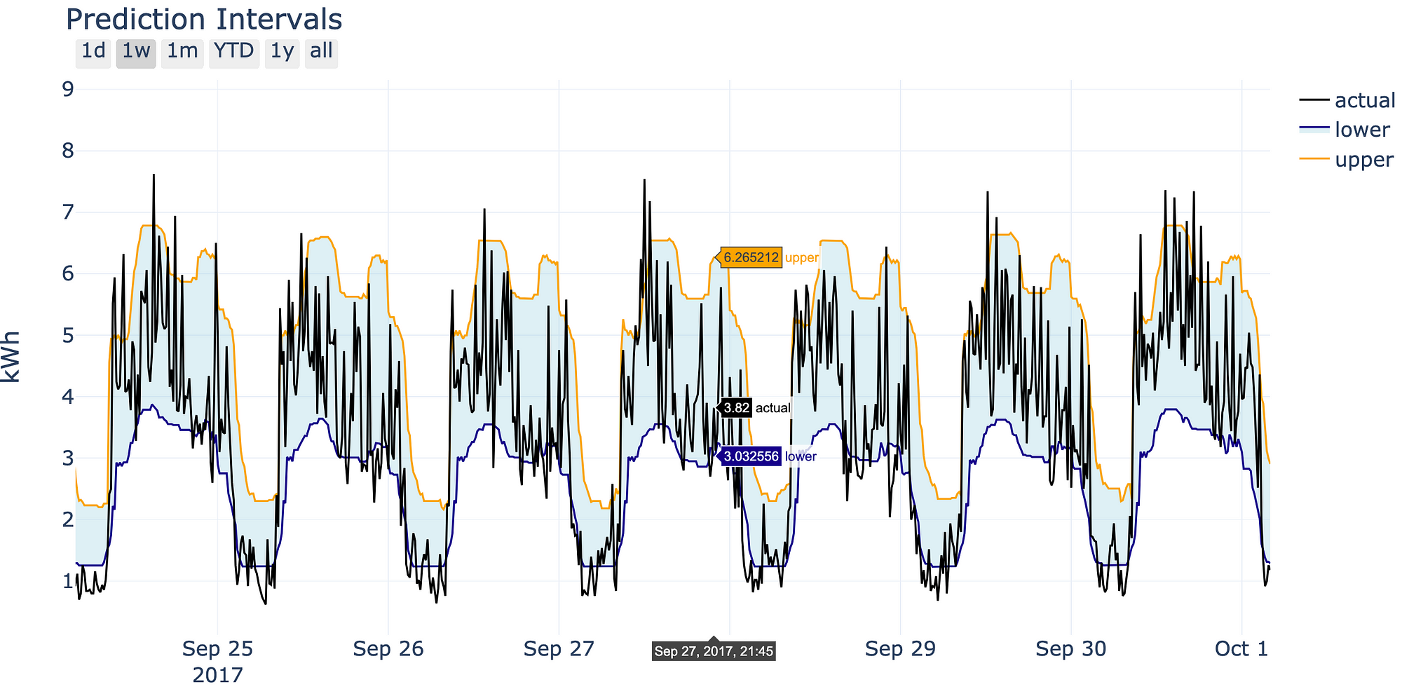Prediction intervals we’ll make in this walkthough.

Problem Set-Up

For this walk-through, we’ll use real-world building energy data from a machine learning competition which was hosted on DrivenData. You can get the raw data here, but I’ve provided a cleaned-up version in GitHub which has energy and eight features measured at 15-minute intervals.

data.head()

Cleaned building energy data

The objective is to predict the energy consumption from the features. (This is an actual task we do every day at Cortex Building Intel!). There are undoubtedly hidden features (latent variables) not captured in our data that affect energy consumption, and therefore, we want to show the uncertainty in our estimates by predicting both an upper and lower bound for energy use.

# Use plotly + cufflinks for interactive plotting
import cufflinks as cf

data.resample('12 H').mean().iplot()

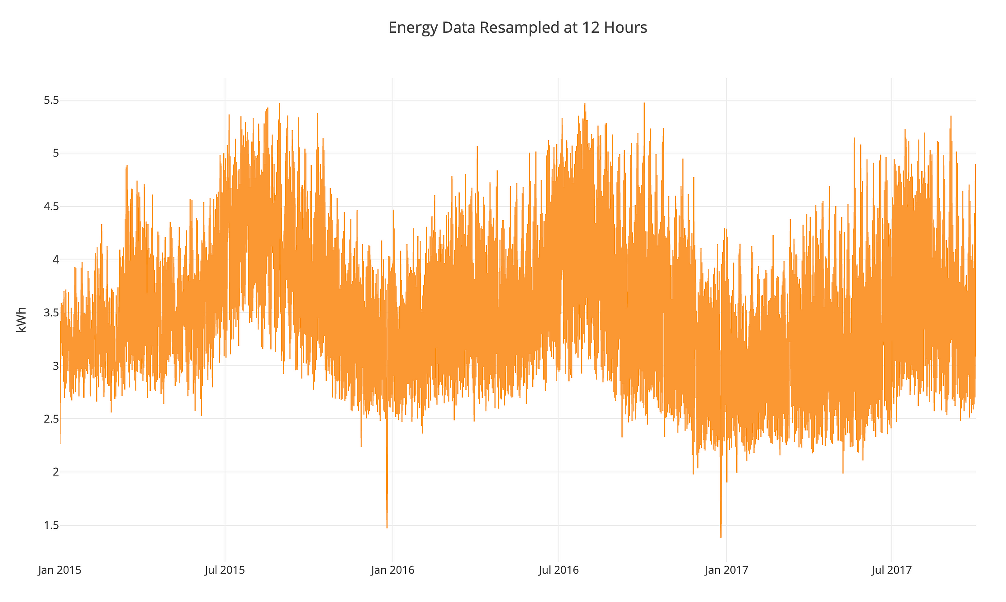Building energy data from DrivenData (hosting machine learning competitions for good!)

Implementation

To generate prediction intervals in Scikit-Learn, we’ll use the Gradient Boosting Regressor, working from this example in the docs. The basic idea is straightforward:

1. For the lower prediction, use GradientBoostingRegressor(loss= "quantile", alpha=lower_quantile) with lower_quantile representing the lower bound, say 0.1 for the 10th percentile
2. For the upper prediction, use the GradientBoostingRegressor(loss= "quantile", alpha=upper_quantile) with upper_quantile representing the upper bound, say 0.9 for the 90th percentile
3. For the mid prediction, use GradientBoostingRegressor(loss="quantile", alpha=0.5) which predicts the median, or the default loss="ls" (for least squares) which predicts the mean. The example in the docs uses the latter approach, and so will we.

At a high level, the loss is the function optimized by the model. When we change the loss to quantile and choose alpha (the quantile), we’re able to get predictions corresponding to percentiles. If we use lower and upper quantiles, we can produce an estimated range. (We won’t get into the details on the quantile loss right here — see the background on Quantile Loss below.)

After splitting the data into train and test sets, we build the model. We actually have to use 3 separate Gradient Boosting Regressors because each model is optimizing a different function and must be trained separately.

from sklearn.ensemble import GradientBoostingRegressor

# Set lower and upper quantile
LOWER_ALPHA = 0.1
UPPER_ALPHA = 0.9

# Each model has to be separate
lower_model = GradientBoostingRegressor(loss="quantile",
                                        alpha=LOWER_ALPHA)
# The mid model will use the default loss
mid_model = GradientBoostingRegressor(loss="ls")

upper_model = GradientBoostingRegressor(loss="quantile",
                                        alpha=UPPER_ALPHA)

Training and predicting uses the familiar Scikit-Learn syntax:

# Fit models
lower_model.fit(X_train, y_train)
mid_model.fit(X_train, y_train)
upper_model.fit(X_train, y_train)

# Record actual values on test set
predictions = pd.DataFrame(y_test)

# Predict
predictions['lower'] = lower_model.predict(X_test)
predictions['mid'] = mid_model.predict(X_test)
predictions['upper'] = upper_model.predict(X_test)

Just like that, we have prediction intervals!

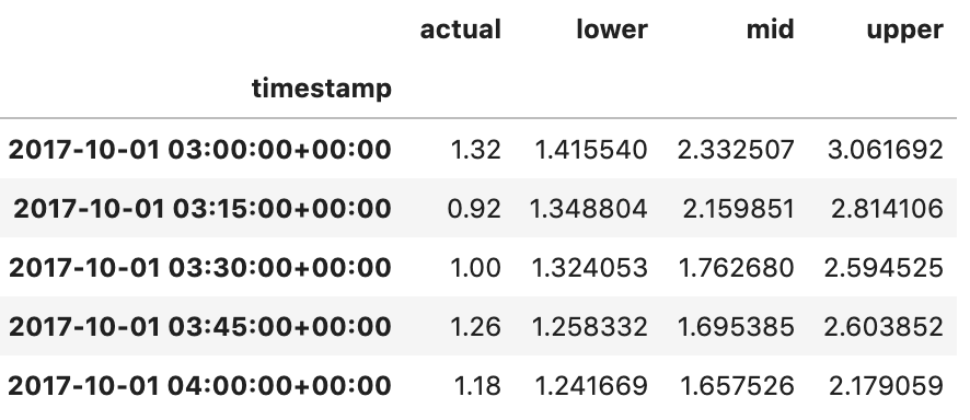Prediction intervals from three Gradient Boosting models Prediction intervals visualized

With a little bit of plotly, we can generate a nice interactive plot.

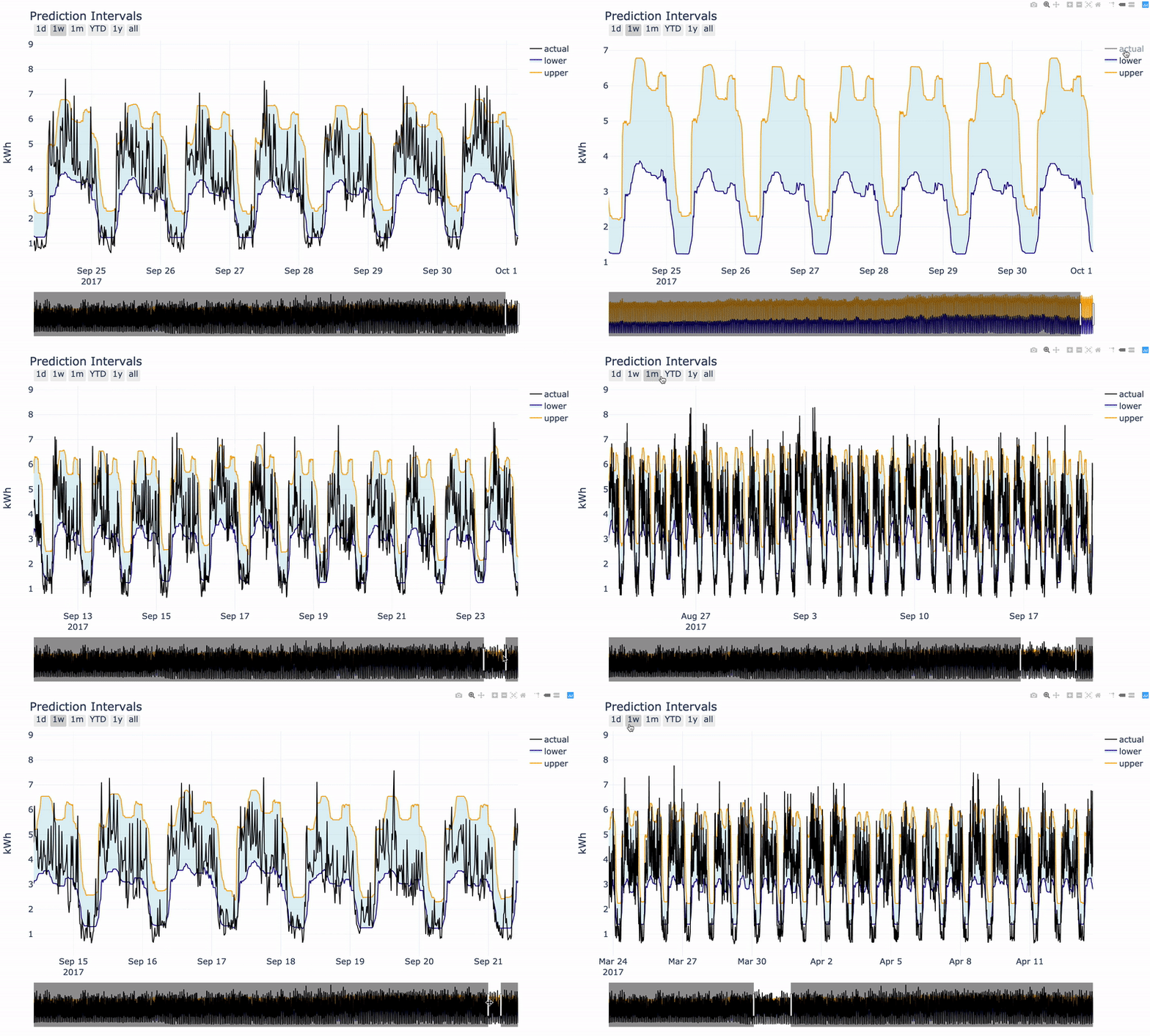Interactive plot produced with plotly

Calculating Prediction Error

As with any machine learning model, we want to quantify the error for our predictions on the test set (where we have the actual answers). Measuring the error of a prediction interval is a little bit trickier than a point prediction. We can calculate the percentage of the time the actual value is within the range, but this can be easily optimized by making the interval very wide. Therefore, we also want a metric that takes into account how far away the predictions are from the actual value, such as absolute error.

In the notebook, I’ve provided a function that calculates the absolute error for the lower, mid, and upper predictions and then averages the upper and lower error for an “Interval” absolute error. We can do this for each data point and then plot a boxplot of the errors (the percent in bounds is in the title):

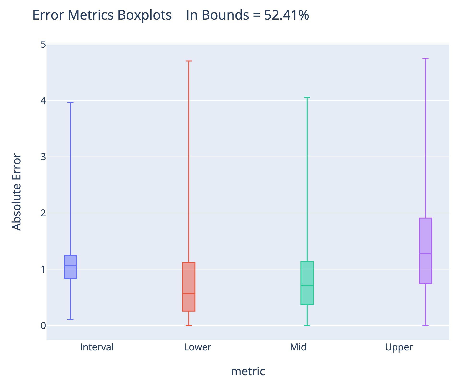Interestingly, for this model, the median absolute error for the lower prediction is actually less than for the mid prediction. This model doesn’t have superb accuracy and could probably benefit from optimization (adjusting model hyperparameters). The actual value is between the lower and upper bounds just over half the time, a metric we could increase by lowering the lower quantile and raising the upper quantile at a loss in precision.

There are probably better metrics, but I selected these because they are simple to calculate and easy to interpret. The actual metrics you use should depend on the problem you’re trying to solve and your objectives.

Prediction Interval Model

Fitting and predicting with 3 separate models is somewhat tedious, so we can write a model that wraps the Gradient Boosting Regressors into a single class. It’s derived from a Scikit-Learn model, so we use the same syntax for training / prediction, except now it’s in one call:

# Instantiate the class
model = GradientBoostingPredictionIntervals(
    lower_alpha=0.1, upper_alpha=0.9
)

# Fit and make predictions
_ = model.fit(X_train, y_train)
predictions = model.predict(X_test, y_test)

The model also comes with some plotting utilities:

fig = model.plot_intervals(mid=True, start='2017-05-26',
                           stop='2017-06-01')
iplot(fig)

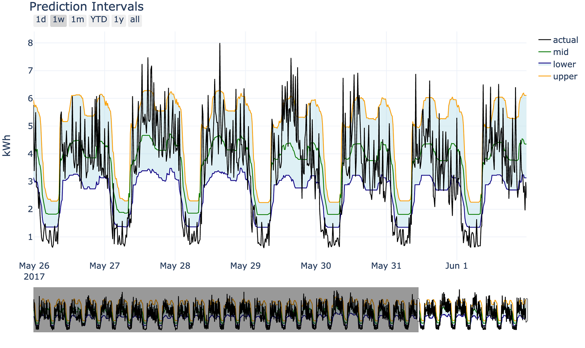Please use and adapt the model as you see fit! This is only one method of making uncertainty predictions, but I think it’s useful because it uses the Scikit-Learn syntax (meaning a shallow learning curve) and we can expand on it as needed. In general, this is a good approach to data science problems: start with the simple solution and add complexity only as required!

Background: Quantile Loss and the Gradient Boosting Regressor

The Gradient Boosting Regressor is an ensemble model, composed of individual decision/regression trees. (For the original explanation of the model, see Friedman’s 1999 paper “Greedy Function Approximation: A Gradient Boosting Machine”.) In contrast to a random forest, which trains trees in parallel, a gradient boosting machine trains trees sequentially, with each tree learning from the mistakes (residuals) of the current ensemble. The contribution of a tree to the model is determined by minimizing the loss function of the model’s predictions and the actual targets in the training set.

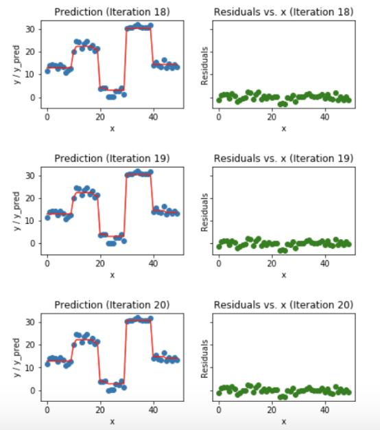Each iteration of the gradient boosting machine trains a new decision/regression tree on the residuals (source)

With the default loss function — least squares — the gradient boosting regressor is predicting the mean. The critical point to understand is that the least squares loss penalizes low and high errors equally:

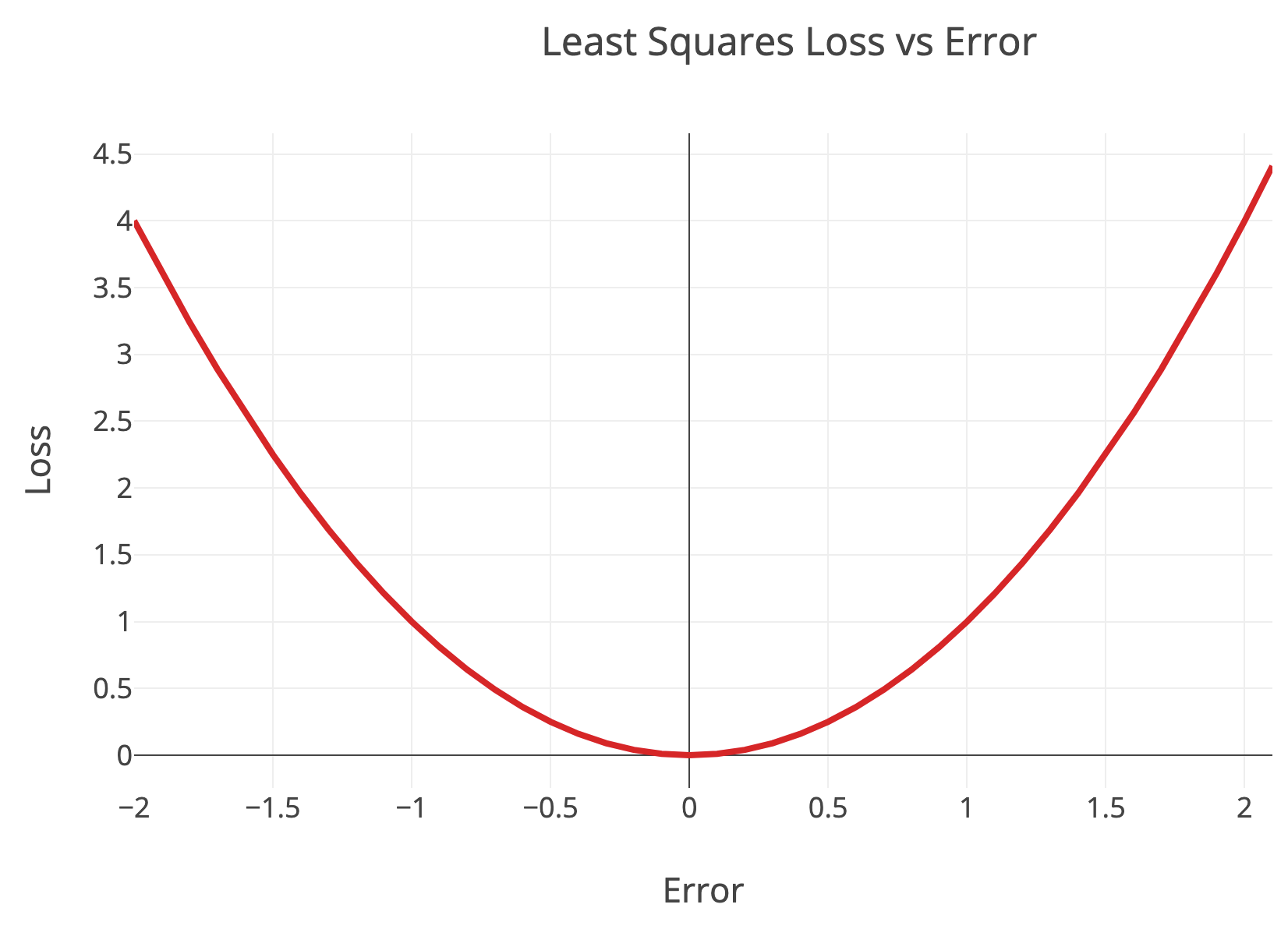Least squares loss versus error

In contrast, the quantile loss penalizes errors based on the quantile and whether the error was positive (actual > predicted) or negative (actual < predicted). This allows the gradient boosting model to optimize not for the mean, but for percentiles. The quantile loss is:

Where α is the quantile. Let’s walk through a quick example using an actual value of 10 and our quantiles of 0.1 and 0.9:

1. If α = 0.1 and predicted = 15, then loss = (0.1–1) * (10–15) = 4.5
2. If α = 0.1 and predicted = 5, then loss = 0.1 * (10–5) = 0.5
3. If α = 0.9 and predicted = 15, then loss = (0.9–1) * (10–15) = 0.5
4. If α = 0.9 and predicted = 5, then loss = 0.9 * (10–5) = 4.5

For a quantile < 0.5, if the prediction is greater than the actual value (case 1), the loss is greater than for a prediction an equal distance above the actual value. For a quantile > 0.5, if the prediction is less than the actual value (case 4), the loss is greater than for a prediction an equal distance below the actual value. With a quantile == 0.5, then predictions above and below the actual value result in an equal error and the model optimizes for the median.

(For the mid model, we can use either loss="quantile", alpha=0.5 for the median, or loss="ls" for the mean).

The quantile loss is best illustrated in a graph showing loss versus error:

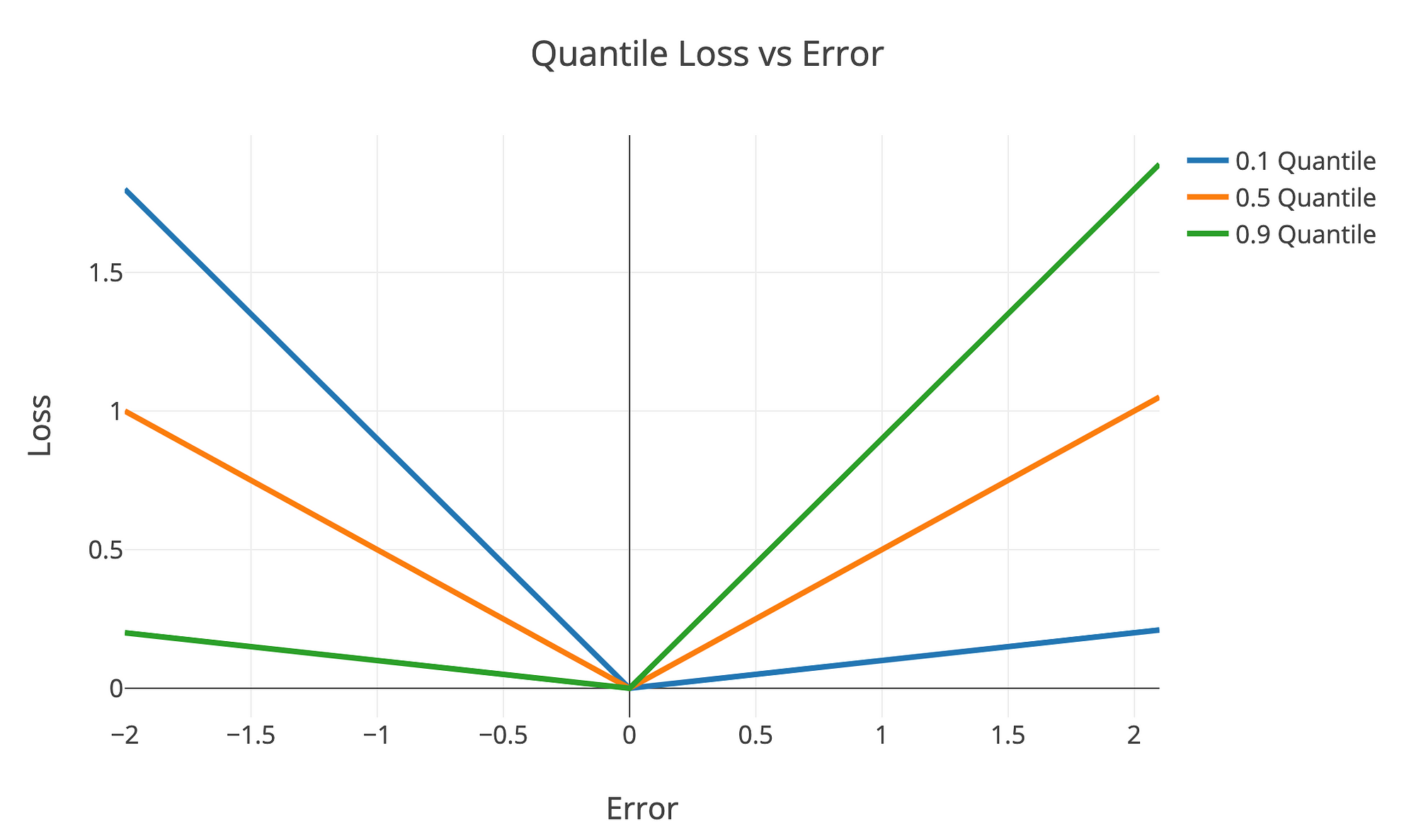Quantile loss versus error for different quantiles

Quantiles < 0.5 drive the predictions below the median and quantiles > 0.5 drive the predictions above the median. This is a great reminder that the loss function of a machine learning method dictates what you are optimizing for!

Depending on the output we want, we can optimize for the mean (least squares), median (quantile loss with alpha == 0.5) , or any percentile (quantile loss with alpha == percentile / 100). This is a relatively simple explanation of the quantile loss, but it’s more than enough to get you started generating prediction intervals with the model walkthrough. To go further, check out this article or start on the Wikipedia page and look into the sources.

Conclusions

Predicting a single number from a machine learning model gives the illusion we have a high level of confidence in the entire modeling process. However, when we remember that any model is only an approximation, we see the need for expressing uncertainty when making estimates. One way to do this is by generating prediction intervals with the Gradient Boosting Regressor in Scikit-Learn. This is only one way to predict ranges (see confidence intervals from linear regression for example), but it’s relatively simple and can be tuned as needed. In this article, we saw a complete implementation and picked up some of the theory behind the quantile loss function.

Solving data science problems is about having many tools in your toolbox to apply as needed. Generating prediction intervals is a helpful technique, and I encourage you to take this walkthrough and apply it to your problems. (The best way to learn any technique is through practice!) We know machine learning can do some pretty incredible things, but it’s not perfect and we shouldn’t portray it as such. To gain the trust of decision-makers, we often need to present not a single number as our estimate, but rather a prediction range indicating the uncertainty inherent in all models.

** * **

I write about Data Science and occasionally other interesting topics. You can follow me on twitter for useful techniques and tools. If saving the world while helping the bottom line appeals to you, then get in touch with us at Cortex.