Exploring financial data with object-oriented programming and additive models

It’s easy to get carried away with the wealth of data and free open-source tools available for data science. After spending a little bit of time with the quandl financial library and the prophet modeling library, I decided to try some simple stock data exploration. Several days and 1000 lines of Python later, I ended up with a complete stock analysis and prediction tool. Although I am not confident (or foolish) enough to use it to invest in individual stocks, I learned a ton of Python in the process and in the spirit of open-source, want to share my results and code so others can benefit.

Now more than ever

This article will show how to use Stocker, a Python class-based tool for stock analysis and prediction (the name was originally arbitrary, but I decided after the fact it nicely stands for “stock explorer”). I had tried several times to conquer classes, the foundation of object-oriented programming in Python, but as with most programming topics, they never quite made sense to me when I read the books. It was only when I was deep in a project faced with a problem I had not solved before that the concept finally clicked, showing once again that experience beats theoretical explanations! In addition to an exploration of Stocker, we will touch on some important topics including the basics of a Python class and additive models. For anyone wanting to use Stocker, the complete code can be found on GitHub along with documentation for usage. Stocker was designed to be easy to use (even for those new to Python), and I encourage anyone reading to try it out. Now, let’s take a look at the analysis capabilities of Stocker!

# Getting Started with Stocker

After installing the required libraries, the first thing we do is import the Stocker class into our Python session. We can do this from an interactive Python session or a Jupyter Notebook started in the directory with the script.

from stocker import Stocker

We now have the Stocker class in our Python session, and we can use it to create an instance of the class. In Python, an instance of a class is called an object, and the act of creating an object is sometimes called instantiation or construction. In order to make a Stocker object we need to pass in the name of a valid stock ticker (bold indicates output).

microsoft = Stocker('MSFT')

**MSFT Stocker Initialized. Data covers 1986-03-13 to 2018-01-16.**

Now, we have a microsoftobject with all the properties of the Stocker class. Stocker is built on the quandl WIKI database which gives us access to over 3000 US stocks with years of daily price data (full list). For this example, we will stick to Microsoft data. Although Microsoft might be seen as the opposite of open-source, they have recently made some changes that make me optimist they are embracing the open-source community (including Python).

A class in Python is comprised of two main parts: attributes and methods. Without going into too much detail, attributes are values or data associated either with the class as a whole or with specific instances (objects) of the class. Methods are functions contained in the class which can act on that data. One attribute of a Stocker object is stock data for a specific company that is attribute is associated with the object when we construct it. We can access the attribute and assign it to another variable for inspection:

# Stock is an attribute of the microsoft object
stock_history = microsoft.stock
stock_history.head()

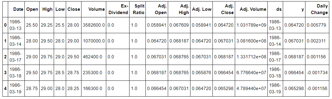Microsoft Stock Data

The benefit of a Python class is that the methods (functions) and the data they act on are associated with the same object. We can use a method of the Stocker object to plot the entire history of the stock.

# A method (function) requires parentheses
microsoft.plot_stock()

**Maximum Adj. Close = 89.58 on 2018-01-12.
Minimum Adj. Close = 0.06 on 1986-03-24.
Current Adj. Close = 88.35.**

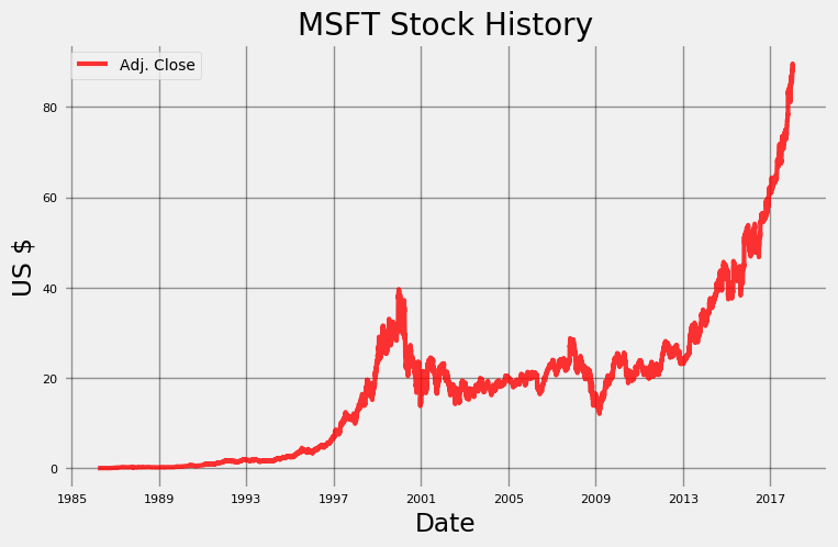The default value plotted is the Adjusted Closing price, which accounts for splits in the stock (when one stock is split into multiple stocks, say 2, with each new stock worth 1/2 of the original price).

This is a pretty basic plot that we could have found from a Google Search, but there is something satisfying about doing it ourselves in a few lines of Python! The plot_stockfunction has a number of optional arguments. By default, this method plots the Adjusted Closing price for the entire date range, but we can choose the range, the stats to plot, and the type of plot. For example, if we want to compare the Daily Change in price with the Adjusted Volume (number of shares) traded, we can specify those in the function call.

microsoft.plot_stock(start_date = '2000-01-03',  end_date = '2018-01-16',  stats = ['Daily Change', 'Adj. Volume'],  plot_type='pct')

**Maximum Daily Change = 2.08 on 2008-10-13.
Minimum Daily Change = -3.34 on 2017-12-04.
Current Daily Change = -1.75.

Maximum Adj. Volume = 591052200.00 on 2006-04-28.
Minimum Adj. Volume = 7425503.00 on 2017-11-24.
Current Adj. Volume = 35945428.00.**

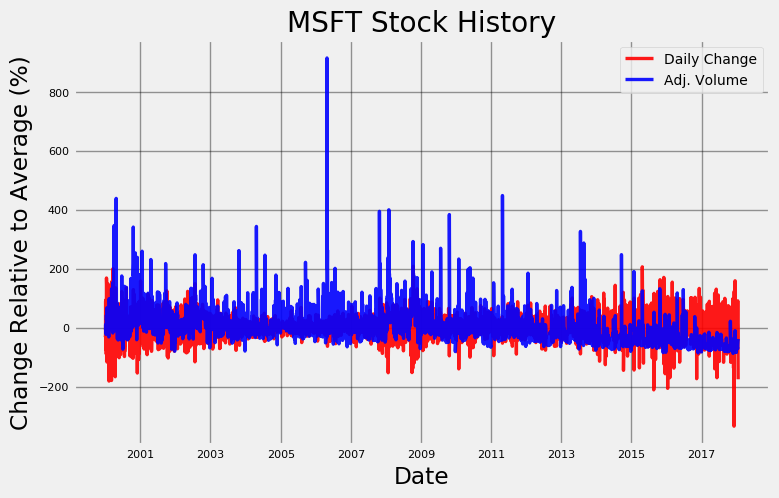Notice the y-axis is in percentage change relative to the average value for the statistic. This scale is necessary because the daily volume is originally in shares, with a range in the hundreds of millions, while daily price change typically is a few dollars! By converting to percentage change we can look at both datasets on a similar scale. The plot shows there is no correlation between the number of shares traded and the daily change in price. This is surprising as we might have expected more shares to be traded on days with larger price changes as people rush to take advantage of the swings. However, the only real trend seems to be that the volume traded decreases over time. There is also a significant decrease in price on December 4, 2017 that we could try to correlate with news stories about Microsoft. A quick news search for December 3 yields the following:

Not sure about the reliability of these sources Google

There certainly does not seem to be any indication that Microsoft stock is due for its largest price decrease in 10 years the next day! In fact, if we were playing the stock market based on news, we might have been tempted to buy stock because a deal with the NFL (second result) sounds like a positive!

Using plot_stock,we can investigate any of the quantities in the data across any date range and look for correlations with real-world events (if there are any). For now, we will move on to one of the more enjoyable parts of Stocker: making fake money!

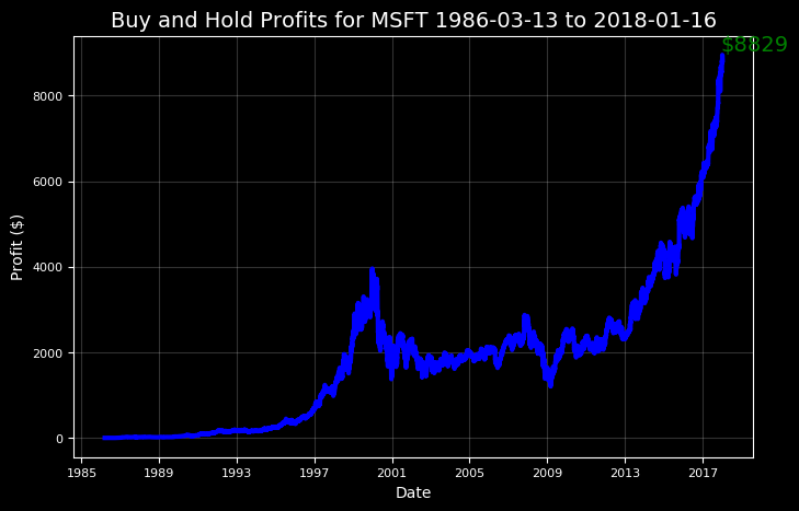
Let’s pretend for a moment we had the presence of mind to invest in 100 shares of Microsoft at the company’s Initial Public Offering (IPO). How much richer would we be now?

microsoft.buy_and_hold(start_date='1986-03-13',
                       end_date='2018-01-16', nshares=100)

**MSFT Total buy and hold profit from 1986-03-13 to 2018-01-16 for 100 shares = $8829.11**

In addition to making us feel better, using these results will allow us to plan our trips back in time to maximize profits.

If we are feeling too confident, we can try to tweak the results to lose money:

microsoft.buy_and_hold(start_date='1999-01-05',
                      end_date='2002-01-03', nshares=100)

**MSFT Total buy and hold profit from 1999-01-05 to 2002-01-03 for 100 shares = $-56.92**

Surprisingly, it is possible to lose money in the stock market!

Additive Models

Additive models are a powerful tool for analyzing and predicting time series, one of the most common types of real world data. The concept is straightforward: represent a time series as a combination of patterns on different time scales and an overall trend. We know the long-term trend of Microsoft stock is a steady increase, but there could also be patterns on a yearly or daily basis, such as an increase every Tuesday, that would be economically beneficial to know. A great library for analyzing time series with daily observations (such as stocks) is Prophet, developed by Facebook. Stocker does all the modeling work with Prophet behind the scenes for us, so we can use a simple method call to create and inspect a model.

model, model_data = microsoft.create_prophet_model()

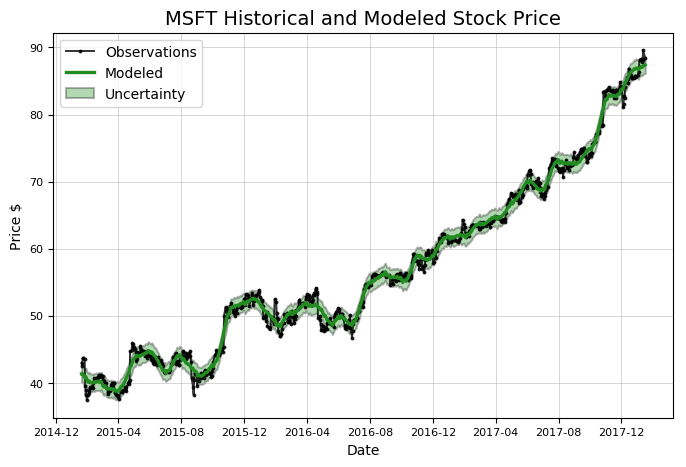The additive model smooths out the noise in the data, which is why the modeled line does not exactly line up with the observations. Prophet models also calculate uncertainty, an essential part of modeling as we can never be sure of our predictions when dealing with fluctuating real life processes. We can also use a prophet model to make predictions for the future, but for now we are more concerned with past data. Notice that this method call returned two objects, a model and some data, which we assigned to variables. We now use these variables to plot the time series components.

# model and model_data are from previous method call
model.plot_components(model_data)
plt.show()

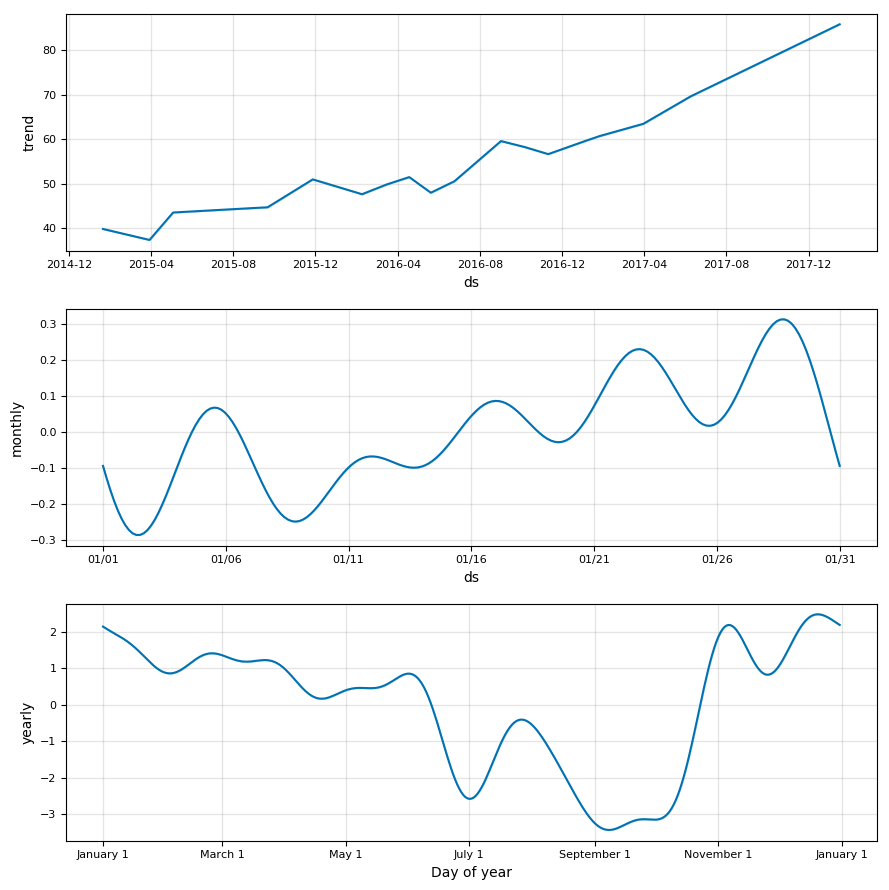The overall trend is a definitive increase over the past three years. There also appears to be a noticeable yearly pattern (bottom graph), with prices bottoming out in September and October and reaching a peak in November and January. As the time-scale decreases, the data gets noisier. Over the course of a typical month, there is more signal than noise! If we believe there might be a weekly pattern, we can add that in to the prophet model by changing the weekly_seasonalityattribute of the Stocker object:

print(microsoft.weekly_seasonality)
microsoft.weekly_seasonality = True
print(microsoft.weekly_seasonality)

**False
True**

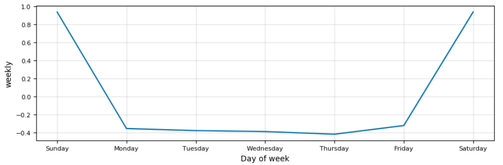
The default value for weekly_seasonalityis False, but we changed the value to include a weekly pattern in our model. We then make another call to create_prophet_modeland graph the resulting components. Below is the weekly seasonality from the new model.

There was no way I could make this graph look good

We can ignore the weekends because the price only changes over the week (in reality the price changes by a small amount during after-hours training but it does not affect our analysis). Unfortunately, there is not a trend over the week that we can use and before we continue modeling, we will turn off the weekly seasonality. This behavior is expected: with stock data, as the time scale decreases, the noise starts to wash out the signal. On a day-to-day basis, the movements of stocks are essentially random, and it is only by zooming out to the yearly scale that we can see trends. Hopefully this serves as a good reminder of why not to play the daily stock game!

Changepoints

Changepoints occur when a time-series goes from increasing to decreasing or vice versa (in a more rigorous sense, they are located where the change in the rate of the time series is greatest). These times are extremely important because knowing when a stock will reach a peak or is about to take off could have significant economic benefits. Identifying the causes of changepoints might let us predict future swings in the value of a stock. The Stocker object can automatically find the 10 largest changepoints for us.

microsoft.changepoint_date_analysis()

**Changepoints sorted by slope rate of change (2nd derivative):

          Date  Adj. Close     delta
48  2015-03-30   38.238066  2.580296
337 2016-05-20   48.886934  2.231580
409 2016-09-01   55.966886 -2.053965
72  2015-05-04   45.034285 -2.040387
313 2016-04-18   54.141111 -1.936257**

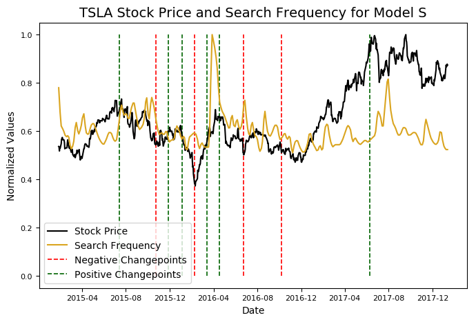
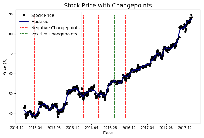The changepoints tend to line up with peaks and valleys in the stock price. Prophet only finds changepoints in the first 80% of the data, but nonetheless, these results are useful because we can attempt to correlate them with real-world events. We could repeat what we did earlier and manually search for Google News around these dates, but I thought it would be preferable if Stocker did that for us. You might have seen the Google Search Trends tool which allows you to see the popularity of any search term over time in Google searches. Stocker can automatically retrieve this data for any search term we specify and plot the result on the original data. To find and graph the frequency of a search term, we modify the previous method call.

# same method but with a search term
microsoft.changepoint_date_analysis(search = 'Microsoft profit')

**Top Related Queries:

                  query  value
0  microsoft non profit    100
1      microsoft office     55
2                 apple     30
3         microsoft 365     30
4  microsoft office 365     20

 Rising Related Queries:

                   query  value
0          microsoft 365    120
1   microsoft office 365     90
2  microsoft profit 2014     70**

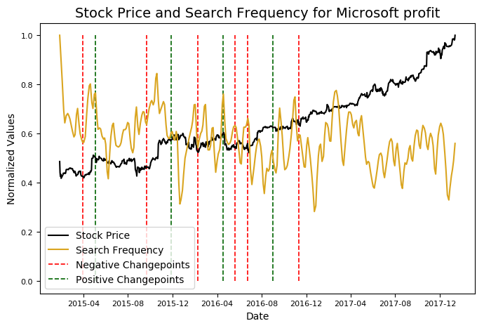In addition to graphing the relative search frequency, Stocker displays the top related queries and the top rising queries for the date range of the graph. On the graph, the y-axis is normalized between 0 and 1 by dividing the values by their maximums, allowing us to compare two variables with different scales. From the figure, there does not appear to be a correlation between searches for “Microsoft profit” and the stock price of Microsoft.

Had we found a correlation, there would still be the question of causation. We would not know if searches or news caused the price to change, or if the change in price caused the searches. There might be some useful information to be found, but there are also many chance correlations. (For a humorous take on such random relationships, check out spurious correlations). Feel free to try out some different terms to see if you can find any interesting trends!

microsoft.changepoint_date_analysis(search = 'Microsoft Office')

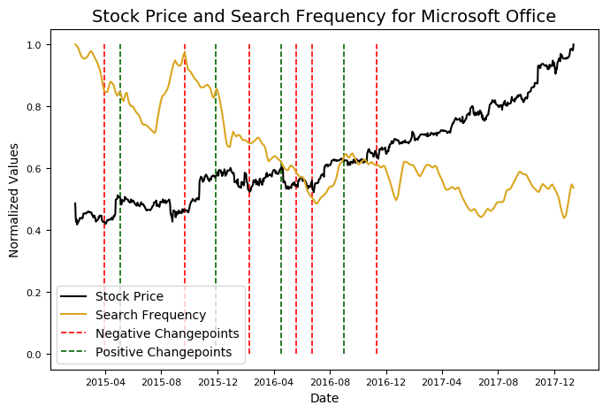Looks like declining searches for Office leads to increasing stock prices. Maybe someone should let Microsoft know.

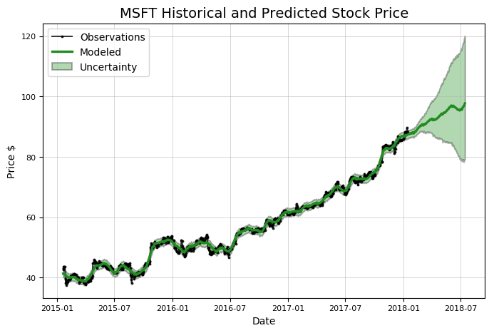
Predictions

We have only explored the first half of Stocker capabilities. The second half is designed for forecasting, or predicting future stock price. Although this might be a futile exercise (or at least will not pay off), there is still plenty to learn in the process! Stay tuned for a future article on prediction, or get started predicting with Stocker on your own (check out the documentation for details). For now, I’ll leave you with one more image.

# specify number of days in future to make a prediction
model, future = microsoft.create_prophet_model(days=180)

**Predicted Price on 2018-07-15 = $97.67**

Although all the capabilities of Stocker might already be publically available, the process of creating this tool was enjoyable, and more importantly, taught me more about data science, Python, and the stock market than any college course could. We live in an incredible age of democratized knowledge where anyone can learn about programming or even state of the art fields like machine learning without formal instruction. If you have an idea for a project but think you do not know enough or find out it has been done before, don’t let that stop you. You might develop a better solution and even if you don’t, you’ll be better off and know more than if you had never started!

As always, I welcome constructive criticism and feedback. I can be reached on twitter at @koehrsen_will.