(Source)

Means, Medians, and Skewed Distributions in the Real World

Most people see the headline “90% of Drivers Consider Themselves Above Average” and think “wow, other people are terrible at evaluating themselves objectively.” What you should think is “that doesn’t sound so implausible if we’re using the mean for average in a heavily negative-skewed distribution.”

Although a headline like this is often used to illustrate the illusion of superiority, (where people overestimate their competence) it also provides a useful lesson in clarifying your assertions when you talk statistics about data. In this particular case, we need to differentiate between the mean and median of a set of values. Depending on the question we ask, it is possible for 9/10 drivers to be above average. Here’s the data to prove it:

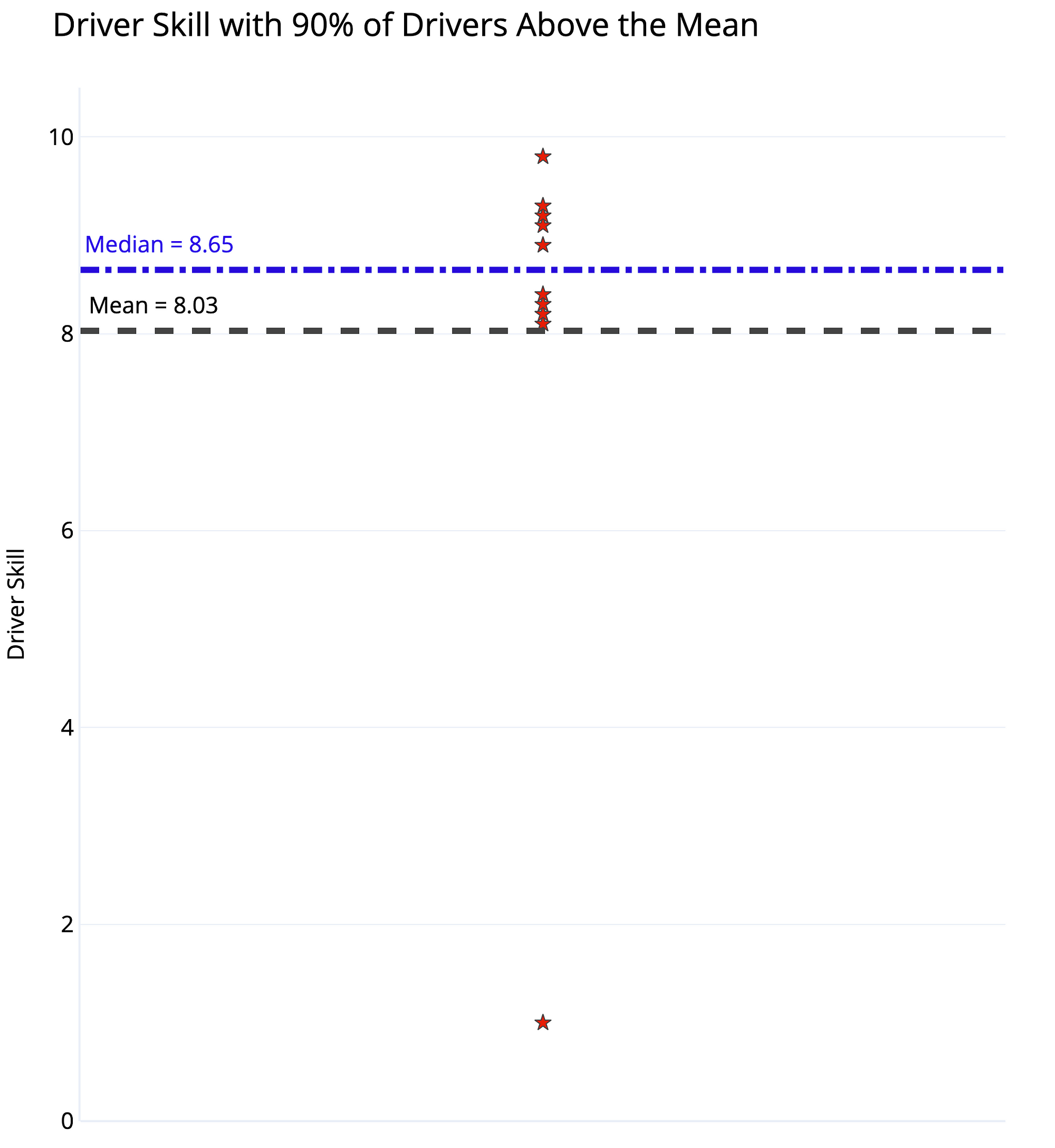Driver Skill Dataset and Dot Plot with Mean and Median

The distinction is whether we use mean or median for “average” driver skill. Using the mean, we add up all the values and divide by the number of values, giving us 8.03 for this dataset. Since 9 of the 10 drivers have a skill rating greater than this, 90% of the drivers could be considered above average!

The median, in contrast, is found by ordering the values from lowest to highest and selecting the value where half the data points are smaller and half are larger. Here it’s 8.65 with 5 drivers below and 5 above. By definition, 50% of drivers are below the median and 50% exceed the median. If the question is “do you consider yourself better than 50% of other drivers?” than 90+% of drivers cannot truthfully answer in the affirmative.

(The median is a particular case of a percentile (also called a quantile), a value at which the given % of numbers are smaller. The median is the 50th quantile: 50% of numbers in a dataset are smaller. We could also find the 90th quantile, where 90% of values are smaller or the 10th quantile, where 10% of values are smaller. Percentiles are an intuitive way to describe a dataset.)

Why Does This Matter?

This might appear to be a contrived example or a technicality, but data where the mean and median are not in agreement come up often in the real world. The mean is equal to the median when values are symmetrically distributed. However, real-world datasets almost always have a measure of skew, either positive or negative:

Positive, symmetric, and negative skews. (Source)

In a positively skewed distribution, the mean is greater than the median. This occurs when a relatively few number of outliers on the upper end of the graph “skew” it rightward, while the majority of the values are clustered at lower values. A real-world situation is personal income, where the mean income is significantly greater than the median income. The following plot shows the US income distribution in 2017 as 100 percentiles in a histogram.

Income distribution in the United States, a positively skewed distribution

The exact numbers vary by source (this data is from here) but the overall pattern is clear: a few very high earners skew the graph towards the right (positive) raising the mean above the median. At a value of $55880, the mean is close to the 66th percentile. The interpretation is 66% of Americans make less than the average national income — when the average is taken to be the mean! This phenomenon occurs in nearly every country.

An example of a negatively skewed distribution is age at death. In this dataset, there are, unfortunately, some deaths at a relatively young age, lowering the mean and skewing the graph leftward (negatively).

Age at death in Australia, a negatively skewed distribution (Source)

In the case of a negative skew, the median is greater than the mean. The result is that more people can be above the “average” when the average is defined as mean. “Majority of people live longer than average” might be a strange headline, but if you choose your stats carefully, you can make it true.

Most datasets involving human behavior exhibit some kind of skew. Stock market returns, income, social media followers, battle deaths, and sizes of cities are all highly skewed distributions. In Antifragile, Nassim Taleb describes this world of skewed outcomes as extremistan. We evolved in mediocristan, where all datasets are normally distributed, but our modern lives are now dominated by unequal distributions. Living in extremistan presents opportunities for incredible rewards, but these will only accrue to a very small number of people. It also means we have to be careful when talking about means and medians as the “average” representation of a dataset.

DIstribution of Followers (source) on social media, a positively skewed distribution.

(Zip’s Law and other power laws also produce skewed distributions.)

Conclusions

The point to remember is when you specify “average”, you need to clarify whether you are talking about the mean or the median because it makes a difference. The world is not symmetrically distributed, and, therefore, we should not expect the mean and median of a distribution to be the same.

Machine learning may get all the attention, but the really important parts of data science are those we use every day: basic statistics to help us understand the world. Being able to tell the difference between a mean and a median may seem mundane, but it’ll be a lot more relevant to your daily life than knowing how to build a neural network.

As always, I welcome feedback and constructive criticism. I can be reached on Twitter @koehrsen_will.