
A Data Science for Good Machine Learning Project Walk-Through in Python: Part Two
Getting the most from our model, figuring out what it all means, and experimenting with new techniques
Machine learning is a powerful framework that from the outside may look complex and intimidating. However, once we break down a problem into its component steps, we see that machine learning is really only a sequence of understandable processes, each one simple by itself.
In the first half of this series, we saw how we could implement a solution to a “data science for good” machine learning problem, leaving off after we had selected the Gradient Boosting Machine as our model of choice.
 Model evaluation results from part one.
In this article, we’ll continue with our pipeline for predicting poverty in Costa Rica, performing model optimizing, interpreting the model, and trying out some experimental techniques.
The full code is available as a Jupyter Notebook both on Kaggle (where it can be run in the browser with no downloads required) and on GitHub. This is an active Kaggle competition and a great project to get started with machine learning or to work on some new skills.
Model Optimization
Model optimization means searching for the model hyperparameters that yield the best performance — measured in cross-validation — for a given dataset. Because the optimal hyperparameters vary depending on the data, we have to optimize — also known as tuning — the model for our data. I like to think of tuning as finding the best settings for a machine learning model.
There are 4 main methods for tuning, ranked from least efficient (manual) to most efficient (automated).
- Manual Tuning: select hyperparameters with intuition/experience or by guessing, train the models with the values, find the validation score, and repeat until you run out of patience or are satisfied with the results.
- Grid Search: set up a hyperparameter grid and for every single combination of values, train a model, and find the validation score. The optimal set of hyperparameters are the ones that score the highest.
- Random Search: set up a hyperparameter grid and select random combinations of values, train the model, and find the validation score. Search iterations are limited based on time/resources
- Automated Tuning: Use methods (gradient descent, Bayesian Optimization, evolutionary algorithms) for a guided search for the best hyperparameters. These are informed methods that use past information.
Naturally, we’ll skip the first three methods and move right to the most efficient: automated hyperparameter tuning. For this implementation, we can use the Hyperopt library, which does optimization using a version of Bayesian Optimization with the Tree Parzen Estimator. You don’t need to understand these terms to use the model, although I did write a conceptual explanation here. (I also wrote an article for using Hyperopt for model tuning here.)
The details are a little protracted (see the notebook), but we need 4 parts for implementing Bayesian Optimization in Hyperopt
- Objective function: what we want to maximize (or minimize)
- Domain space: region over which to search
- Algorithm for choosing the next hyperparameters: uses the past results to suggest next values to evaluate
- Results history: saves the past results
The basic idea of Bayesian Optimization (BO) is that the algorithm reasons from the past results — how well previous hyperparameters have scored — and then chooses the next combination of values it thinks will do best. Grid or random search are uninformed methods that don’t use past results and the idea is that by reasoning, BO can find better values in fewer search iterations.
See the notebook for the complete implementation, but below are the optimization scores plotted over 100 search iterations.
 Model optimization scores versus iteration.
Unlike in random search where the scores are, well random over time, in Bayesian Optimization, the scores tend to improve over time as the algorithm learns a probability model of the best hyperparameters. The idea of Bayesian Optimization is that we can optimize our model (or any function) quicker by focusing the search on promising settings. Once the optimization has finished running, we can use the best hyperparameters to cross validate the model.
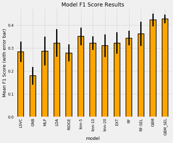
Optimizing the model will not always improve our test score because we are optimizing for the training data. However, sometimes it can deliver a large benefit compared to the default hyperparameters. In this case, the final cross validation results are shown below in dataframe form:
 Cross validation results. Models without 10Fold in name were validated with 5 folds. SEL is selected features.
The optimized model (denoted by OPT and using 10 cross validation folds with the features after selection) places right in the middle of the non-optimized variations of the Gradient Boosting Machine (which used hyperparameters I had found worked well for previous problems.) This indicates we haven’t found the optimal hyperparameters yet, or there could be multiple sets of hyperparameters that performly roughly the same.
We can continue optimization to try and find even better hyperparameters, but usually the return to hyperparameter tuning is much less than the return to feature engineering. At this point we have a relatively high-performing model and we can use this model to make predictions on the test data. Then, since this is a Kaggle competition, we can submit the predictions to the leaderboard. Doing this gets us into the top 50 (at the moment) which is a nice vindication of all our hard work!
At this point, we have implemented a complete solution to this machine learning problem. Our model can make reasonably accurate predictions of poverty in Costa Rican households (the F1 score is relatively low, but this is a difficult problem). Now, we can move on to interpreting our predictions and see if our model can teach us anything about the problem. Even though we have a solution, we don’t want to lose sight of why our solution matters.
Note about Kaggle Competitions
The very nature of machine learning competitions can encourage bad practices, such as the mistake of optimizing for the leaderboard score at the cost of all other considerations. Generally this leads to using ever more complex models to eke out a tiny performance gain.
In the real-world, above a certain threshold — which depends on the application — accuracy becomes secondary to explainability, and you’re better off with a slightly less performant model if it is simpler.
A simple model that is put in use is better than a complex model which can never be deployed. Moreover, those at the top of the leaderboard are probably overfitting to the testing data and do not have a robust model.
A good strategy for getting the most out of Kaggle is to work at a problem until you have a reasonably good solution — say 90% of the top leaderboard scores — and then not stress about getting to the very top. Competing is fun, but learning is the most valuable aspect of taking on these projects.
Interpret Model Results
In the midst of writing all the machine learning code, it can be easy to lose sight of the important questions: what are we making this model for? What will be the impact of our predictions? Thankfully, our answer this time isn’t “increasing ad revenue” but, instead, effectively predicting which households are most at risk for poverty in Costa Rica so they can receive needed help.
To try and get a sense of our model’s output, we can examine the prediction of poverty levels on a household basis for the test data. For the test data, we don’t know the true answers, but we can compare the relative frequency of each predicted class with that in the training labels. The image below shows the training distribution of poverty on the left, and the predicted distribution for the testing data on the right:
 Training label distribution (left) and predicted test distribution (right). Both histograms are normalized.
Intriguingly, even though the label “not vulnerable” is most prevalent in the training data, it is represented less often on a relative basis for the predictions. Our model predicts a higher proportion of the other 3 classes, which means that it thinks there is more severe poverty in the testing data. If we convert these fractions to numbers, we have 3929 households in the “non vulnerable” category and 771 households in the “extreme” category.
Another way to look at the predictions is by the confidence of the model. For each prediction on the test data, we can see not only the label, but also the probability given to it by the model. Let’s take a look at the confidence by the value of the label in a boxplot.
 Boxplot of probability assigned to each label on testing data.
These results are fairly intuitive — our model is most confident in the most extreme predictions — and less confident in the moderate ones. Theoretically, there should be more separation between the most extreme labels and the targets in the middle should be more difficult to tease apart.
Another point to draw from this graph is that overall, our model is not very sure of the predictions. A guess with no data would place 0.25 probability on each class, and we can see that even for the least extreme poverty, our model rarely has more than 40% confidence. What this tells us is this is a tough problem — there is not much to separate the classes in the available data.
Ideally, these predictions, or those from the winning model in the competition, will be used to determine which families are most likely to need assistance. However, just the predictions alone do not tell us what may lead to the poverty or how our model “thinks”. While we can’t completely solve this problem yet, we can try to peer into the black box of machine learning.
In a tree-based model — such as the Gradient Boosting Machine — the feature importances represent the sum total reduction in gini impurity for nodes split on a feature. I never find the absolute values very helpful, but instead normalize the numbers and look at them on a relative basis. For example, below are the 10 most important features from the optimized GBM model.
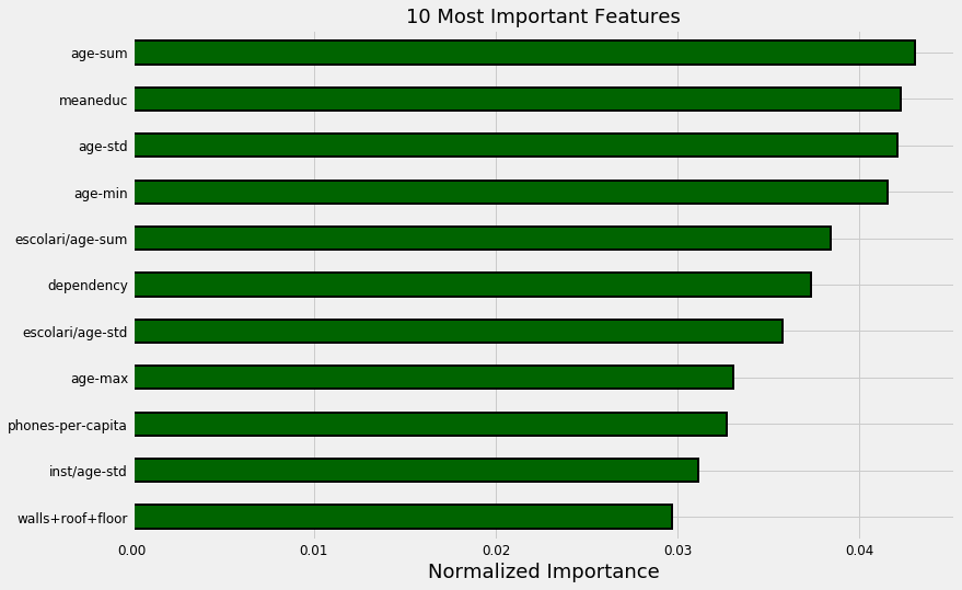 Most important features from optimized gradient boosting machine.
Here we can see education and ages of family members making up the bulk of the most important features. Looking further into the importances, we also see the size of the family. This echoes findings by poverty researchers: family size is correlated to more extreme poverty, and education level is inversely correlated with poverty. In both cases, we don’t necessarily know which causes which, but we can use this information to highlight which factors should be further studied. Hopefully, this data can then be used to further reduce poverty (which has been decreasing steadily for the last 25 years).
 It’s true: the world is better now than ever and still improving (source).
In addition to potentially helping researchers, we can use the feature importances for further feature engineering by trying to build more features on top of these. An example using the above results would be taking the meaneduc and dividing by the dependency to create a new feature. While this may not be intuitive, it’s hard to tell ahead of time what will work for a model.
An alternative method to using the testing data to examine our model is to split the training data into a smaller training set and a validation set. Because we have the labels for all the training data, we can compare our predictions on the holdout validation data to the true values. For example, using 1000 observations for validation, we get the following confusion matrix:
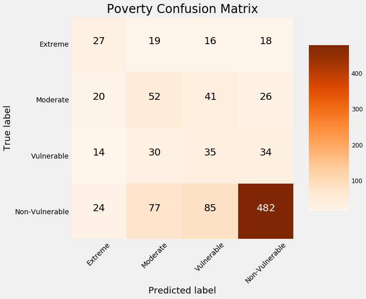 Confusion matrix on validation data.
The values on the diagonal are those the model predicted correctly because the predicted label is the same as the true label. Anything off the diagonal the model predicted incorrectly. We can see that our model is the best at identifying the non-vulnerable households, but is not very good at discerning the other labels.
As one example, our model incorrectly classifies 18 households as non-vulnerable which are in fact in extreme poverty. Predictions like these have real-world consequences because those might be families that as a result of this model, would not receive help. (For more on the consequences of incorrect algorithms, see Weapons of Math Destruction.)
Overall, this mediocre performance — the model accuracy is about 60% which is much better than random guessing but not exceptional — suggests this problem may be difficult. It could be there is not enough information to separate the classes within the available data.
One recommendation for the host organization — the Inter-American Development Bank — is that we need more data to better solve this problem. That could come either in the form of more features — so more questions on the survey — or more observations — a greater number of households surveyed. Either of these would require a significant effort, but the best return to time invested in a data science project is generally by gathering greater quantities of high-quality labeled data.
There are other methods we can use for model understanding, such as Local Interpretable Model-agnostic Explainer (LIME), which uses a simpler linear model to approximate the model around a prediction. We can also look at individual decision trees in a forest which are typically straightforward to parse because they essentially mimic a human decision making process.
 Individual Decision Tree in Random Forest.
Overall, machine learning still suffers from an explainability gap, which hinders its applicability: people want not only accurate predictions, but an understanding of how those predictions were generated.
Exploratory Techniques
We’ve already solved the machine learning problem with a standard toolbox, so why go further into exploratory techniques? Well, if you’re like me, then you enjoy learning new things just for the sake of learning. What’s more, the exploratory techniques of today will be the standard tools of tomorrow.
For this project, I decided to try out two new (to me) techniques:
- Recursive Feature Elimination for feature selection
- Uniform Manifold Approximation and Projection for dimension reduction and visualization
Recursive Feature Elimination
Recursive feature elimination is a method for feature selection that uses a model’s feature importances — a random forest for this application — to select features. The process is a repeated method: at each iteration, the least important features are removed. The optimal number of features to keep is determined by cross validation on the training data.
Recursive feature elimination is simple to use with Scikit-Learn’s RFECV method. This method builds on an estimator (a model) and then is fit like any other Scikit-Learn method. The scorer part is required in order to make a custom scoring metric using the Macro F1 score.
While I’ve used feature importances for selection before, I’d never implemented the Recursive Feature Elimination method, and as usual, was pleasantly surprised at how easy this was to do in Python. The RFECV method selected 58 out of around 190 features based on the cross validation scores:
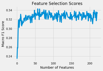 Recursive Feature Elimination Scores.
The selected set of features were then tried out to compare the cross validation performance with the original set of features. (The final results are presented after the next section). Given the ease of using this method, I think it’s a good tool to have in your skill set for modeling. Like any other Scikit-Learn operation, it can fit into a Pipeline, allowing you to quickly execute a complete series of preprocessing and modeling operations.
Dimension Reduction for Visualization
There are a number of unsupervised methods in machine learning for dimension reduction. These fall into two general categories:
- Matrix decomposition algorithms: PCA and ICA
- Embedding techniques that map data onto low-dimension manifolds: IsoMap, t-SNE
Typically, PCA (Principal Components Analysis) and ICA (Independent Components Analysis) are used both for visualization and as a preprocessing step for machine learning, while manifold methods like t-SNE (t-Distributed Stochastic Neighbors Embedding) are used only for visualization because they are highly dependent on hyperparameters and do not preserve distances within the data. (In Scikit-Learn, the t-SNE implementation does not have a transform method which means we can’t use it for modeling).
A new entry on the dimension reduction scene is UMAP: Uniform Manifold Approximation and Projection. It aims to map the data to a low-dimensional manifold — so it’s an embedding technique, while simultaneously preserving global structure in the data. Although the math behind it is rigorous, it can be used like an Scikit-Learn method with a [fit](https://github.com/lmcinnes/umap) and [transform](https://github.com/lmcinnes/umap) call.
I wanted to try these methods for both dimension reduction for visualization, and to add the reduced components as additional features. While this use case might not be typical, there’s no harm in experimenting! Below shows the code for using UMAP to create embeddings of both the train and testing data.
The application of the other three methods is exactly the same (except TSNE which cannot be used to transform the testing data). After completing the transformations, we can visualize the reduced training features in 3 dimensions, with the points colored by the value of the target:
| UMAP | PCA |
|---|---|
 |
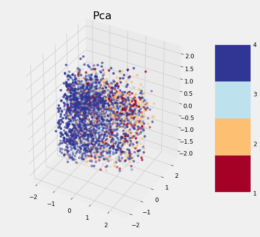 |
| ICA | TSNE |
|---|---|
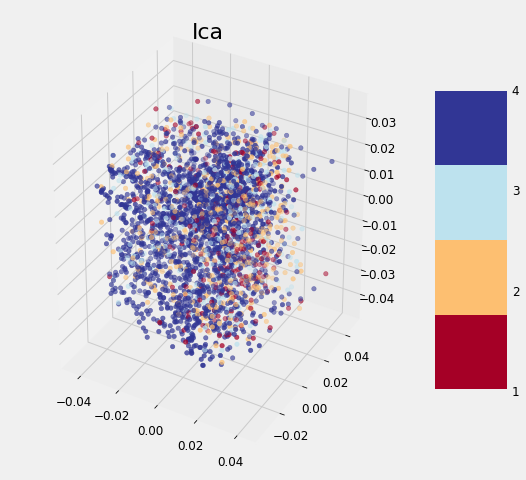 |
 |
None of the methods cleanly separates the data based on the label which follows the findings of other data scientists. As we discovered earlier, it may be that this problem is difficult considering the data to which we have access. Although these graphs cannot be used to say whether or not we can solve a problem, if there is a clean separation, then it indicates that there is something in the data that would allow a model to easily discern each class.
As a final step, we can add the reduced features to the set of features after applying feature selection to see if they are useful for modeling. (Usually dimension reduction is applied and then the model is trained on just the reduced dimensions). The performance of every single model is shown below:
 Final model comparison results.
The model using the dimension reduction features has the suffix DR while the number of folds following the GBM refers to the number of cross validation folds. Overall, we can see that the selected set of features (SEL) does slightly better, and adding in the dimension reduction features hurts the model performance! It’s difficult to conclude too much from these results given the large standard deviations, but we can say that the Gradient Boosting Machine significantly outperforms all other models and the feature selection process improves the cross validation performance.
The experimental part of this notebook was probably the most enjoyable for me. It’s not only important to always be learning to stay ahead in the data science field, but it’s also enjoyable for the sake of learning something new.
The drive to constantly be improving and gaining new knowledge is a critical skill for a data scientist.
Next Steps
Despite this exhaustive coverage of machine learning tools, we have not yet reached the end of methods to apply to this problem!
Some additional steps we could take are:
- Automated Feature Engineering: see this notebook for details
- Oversampling the minority class: a method to account for imbalanced classes by generating synthetic data points
- Further feature selection: especially after automated feature engineering, we have features that could negatively impact model performance
- Ensembling or stacking models: sometimes combining weaker — lower performing — models with stronger models can improve performance
The great part about a Kaggle competition is you can read about many of these cutting-edge techniques in other data scientists’ notebooks. Moreover, these contests give us realistic datasets in a non-mission-critical setting, which is a perfect environment for experimentation.
The best contests can lead to new advances by encouraging friendly competition, open sharing of work, and rewarding innovative approaches.
As one example of the ability of competitions to better machine learning methods, the ImageNet Large Scale Visual Recognition Challenge led to significant improvements in convolutional neural networks.
 Imagenet Competitions have led to state-of-the-art convolutional neural networks.
Conclusions
Data science and machine learning are not incomprehensible methods: instead, they are sequences of straightforward steps that combine into a powerful solution. By walking through a problem one step at a time, we can learn how to build the entire framework. How we use this framework is ultimately up to us. We don’t have to dedicate our lives to helping others, but it is rewarding to take on a challenge with a deeper meaning.
In this article, we saw how we could apply a complete machine learning solution to a data science for good problem, building a machine learning model to predict poverty levels in Costa Rica.
Our approach followed a sequence of processes (1–4 were in part one):
- Understand the problem and data
- Perform data cleaning alongside exploratory data analysis
- Engineer relevant features automatically and manually
- Compare machine learning models
- Optimize the best performing model
- Interpret the model results and explore how it makes predictions
Finally, if after all that you still haven’t got your fill of data science, you can move on to exploratory techniques and learn something new!
As with any process, you’ll only improve as you practice. Competitions are valuable for the opportunities they provide us to employ and develop skills. Moveover, they encourage discussion, innovation, and collaboration, leading both to more capable individual data scientists and a better community. Through this data science project, we not only improve our skills, but also make an effort to improve outcomes for our fellow humans.
As always, I welcome feedback, constructive criticism, and hearing about your data science projects. I can be reached on Twitter @koehrsen_will.