Improving the Random Forest Part Two

So we’ve built a random forest model to solve our machine learning problem (perhaps by following this end-to-end guide) but we’re not too impressed by the results. What are our options? As we saw in the first part of this series, our first step should be to gather more data and perform feature engineering. Gathering more data and feature engineering usually has the greatest payoff in terms of time invested versus improved performance, but when we have exhausted all data sources, it’s time to move on to model hyperparameter tuning. This post will focus on optimizing the random forest model in Python using Scikit-Learn tools. Although this article builds on part one, it fully stands on its own, and we will cover many widely-applicable machine learning concepts.

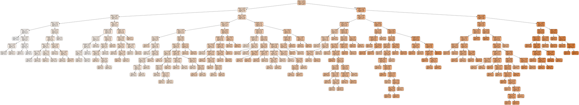One Tree in a Random Forest

I have included Python code in this article where it is most instructive. Full code and data to follow along can be found on the project Github page.

A Brief Explanation of Hyperparameter Tuning

The best way to think about hyperparameters is like the settings of an algorithm that can be adjusted to optimize performance, just as we might turn the knobs of an AM radio to get a clear signal (or your parents might have!). While model parameters are learned during training — such as the slope and intercept in a linear regression — hyperparameters must be set by the data scientist beforetraining. In the case of a random forest, hyperparameters include the number of decision trees in the forest and the number of features considered by each tree when splitting a node. (The parameters of a random forest are the variables and thresholds used to split each node learned during training). Scikit-Learn implements a set of sensible default hyperparameters for all models, but these are not guaranteed to be optimal for a problem. The best hyperparameters are usually impossible to determine ahead of time, and tuning a model is where machine learning turns from a science into trial-and-error based engineering.

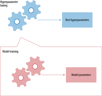Hyperparameters and Parameters

Hyperparameter tuning relies more on experimental results than theory, and thus the best method to determine the optimal settings is to try many different combinations evaluate the performance of each model. However, evaluating each model only on the training set can lead to one of the most fundamental problems in machine learning: overfitting.

If we optimize the model for the training data, then our model will score very well on the training set, but will not be able to generalize to new data, such as in a test set. When a model performs highly on the training set but poorly on the test set, this is known as overfitting, or essentially creating a model that knows the training set very well but cannot be applied to new problems. It’s like a student who has memorized the simple problems in the textbook but has no idea how to apply concepts in the messy real world.

An overfit model may look impressive on the training set, but will be useless in a real application. Therefore, the standard procedure for hyperparameter optimization accounts for overfitting through cross validation.

Cross Validation

The technique of cross validation (CV) is best explained by example using the most common method, K-Fold CV. When we approach a machine learning problem, we make sure to split our data into a training and a testing set. In K-Fold CV, we further split our training set into K number of subsets, called folds. We then iteratively fit the model K times, each time training the data on K-1 of the folds and evaluating on the Kth fold (called the validation data). As an example, consider fitting a model with K = 5. The first iteration we train on the first four folds and evaluate on the fifth. The second time we train on the first, second, third, and fifth fold and evaluate on the fourth. We repeat this procedure 3 more times, each time evaluating on a different fold. At the very end of training, we average the performance on each of the folds to come up with final validation metrics for the model.

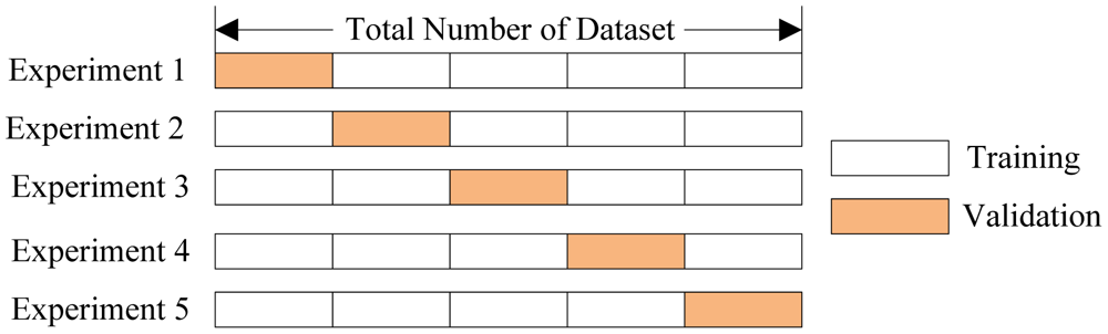5 Fold Cross Validation (Source)

For hyperparameter tuning, we perform many iterations of the entire K-Fold CV process, each time using different model settings. We then compare all of the models, select the best one, train it on the full training set, and then evaluate on the testing set. This sounds like an awfully tedious process! Each time we want to assess a different set of hyperparameters, we have to split our training data into K fold and train and evaluate K times. If we have 10 sets of hyperparameters and are using 5-Fold CV, that represents 50 training loops. Fortunately, as with most problems in machine learning, someone has solved our problem and model tuning with K-Fold CV can be automatically implemented in Scikit-Learn.

Random Search Cross Validation in Scikit-Learn

Usually, we only have a vague idea of the best hyperparameters and thus the best approach to narrow our search is to evaluate a wide range of values for each hyperparameter. Using Scikit-Learn’s RandomizedSearchCV method, we can define a grid of hyperparameter ranges, and randomly sample from the grid, performing K-Fold CV with each combination of values.

As a brief recap before we get into model tuning, we are dealing with a supervised regression machine learning problem. We are trying to predict the temperature tomorrow in our city (Seattle, WA) using past historical weather data. We have 4.5 years of training data, 1.5 years of test data, and are using 6 different features (variables) to make our predictions. (To see the full code for data preparation, see the notebook).

Let’s examine the features quickly.

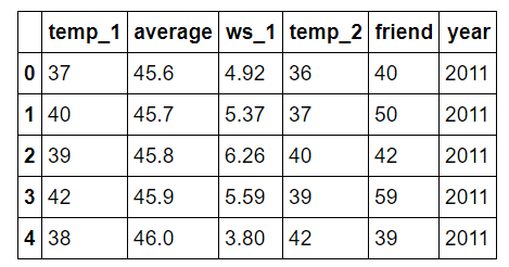Features for Temperature Prediction

• temp_1 = max temperature (in F) one day prior
• average = historical average max temperature
• ws_1 = average wind speed one day prior
• temp_2 = max temperature two days prior
• friend = prediction from our “trusty” friend
• year = calendar year

In previous posts, we checked the data to check for anomalies and we know our data is clean. Therefore, we can skip the data cleaning and jump straight into hyperparameter tuning.

To look at the available hyperparameters, we can create a random forest and examine the default values.

from sklearn.ensemble import RandomForestRegressor

rf = RandomForestRegressor(random_state = 42)

from pprint import pprint

# Look at parameters used by our current forest
print('Parameters currently in use:\n')
pprint(rf.get_params())

**Parameters currently in use:

{'bootstrap': True,
 'criterion': 'mse',
 'max_depth': None,
 'max_features': 'auto',
 'max_leaf_nodes': None,
 'min_impurity_decrease': 0.0,
 'min_impurity_split': None,
 'min_samples_leaf': 1,
 'min_samples_split': 2,
 'min_weight_fraction_leaf': 0.0,
 'n_estimators': 10,
 'n_jobs': 1,
 'oob_score': False,
 'random_state': 42,
 'verbose': 0,
 'warm_start': False}**

Wow, that is quite an overwhelming list! How do we know where to start? A good place is the documentation on the random forest in Scikit-Learn. This tells us the most important settings are the number of trees in the forest (n_estimators) and the number of features considered for splitting at each leaf node (max_features). We could go read the research papers on the random forest and try to theorize the best hyperparameters, but a more efficient use of our time is just to try out a wide range of values and see what works! We will try adjusting the following set of hyperparameters:

• n_estimators = number of trees in the foreset
• max_features = max number of features considered for splitting a node
• max_depth = max number of levels in each decision tree
• min_samples_split = min number of data points placed in a node before the node is split
• min_samples_leaf = min number of data points allowed in a leaf node
• bootstrap = method for sampling data points (with or without replacement)

Random Hyperparameter Grid

To use RandomizedSearchCV, we first need to create a parameter grid to sample from during fitting:

from sklearn.model_selection import RandomizedSearchCV

# Number of trees in random forest
n_estimators = [int(x) for x in np.linspace(start = 200, stop = 2000, num = 10)]
# Number of features to consider at every split
max_features = ['auto', 'sqrt']
# Maximum number of levels in tree
max_depth = [int(x) for x in np.linspace(10, 110, num = 11)]
max_depth.append(None)
# Minimum number of samples required to split a node
min_samples_split = [2, 5, 10]
# Minimum number of samples required at each leaf node
min_samples_leaf = [1, 2, 4]
# Method of selecting samples for training each tree
bootstrap = [True, False]

# Create the random grid
random_grid = {'n_estimators': n_estimators,
               'max_features': max_features,
               'max_depth': max_depth,
               'min_samples_split': min_samples_split,
               'min_samples_leaf': min_samples_leaf,
               'bootstrap': bootstrap}

pprint(random_grid)

**{'bootstrap': [True, False],
 'max_depth': [10, 20, 30, 40, 50, 60, 70, 80, 90, 100, None],
 'max_features': ['auto', 'sqrt'],
 'min_samples_leaf': [1, 2, 4],
 'min_samples_split': [2, 5, 10],
 'n_estimators': [200, 400, 600, 800, 1000, 1200, 1400, 1600, 1800, 2000]}**

On each iteration, the algorithm will choose a difference combination of the features. Altogether, there are 2 * 12 * 2 * 3 * 3 * 10 = 4320 settings! However, the benefit of a random search is that we are not trying every combination, but selecting at random to sample a wide range of values.

Random Search Training

Now, we instantiate the random search and fit it like any Scikit-Learn model:

# Use the random grid to search for best hyperparameters
# First create the base model to tune
rf = RandomForestRegressor()
# Random search of parameters, using 3 fold cross validation,
# search across 100 different combinations, and use all available cores
rf_random = RandomizedSearchCV(estimator = rf, param_distributions = random_grid, n_iter = 100, cv = 3, verbose=2, random_state=42, n_jobs = -1)

# Fit the random search model
rf_random.fit(train_features, train_labels)

The most important arguments in RandomizedSearchCV are n_iter, which controls the number of different combinations to try, and cv which is the number of folds to use for cross validation (we use 100 and 3 respectively). More iterations will cover a wider search space and more cv folds reduces the chances of overfitting, but raising each will increase the run time. Machine learning is a field of trade-offs, and performance vs time is one of the most fundamental.

We can view the best parameters from fitting the random search:

rf_random.best_params_

**{'bootstrap': True,
 'max_depth': 70,
 'max_features': 'auto',
 'min_samples_leaf': 4,
 'min_samples_split': 10,
 'n_estimators': 400}**

From these results, we should be able to narrow the range of values for each hyperparameter.

Evaluate Random Search

To determine if random search yielded a better model, we compare the base model with the best random search model.

def evaluate(model, test_features, test_labels):
    predictions = model.predict(test_features)
    errors = abs(predictions - test_labels)
    mape = 100 * np.mean(errors / test_labels)
    accuracy = 100 - mape
    print('Model Performance')
    print('Average Error: {:0.4f} degrees.'.format(np.mean(errors)))
    print('Accuracy = {:0.2f}%.'.format(accuracy))

    return accuracy

base_model = RandomForestRegressor(n_estimators = 10, random_state = 42)
base_model.fit(train_features, train_labels)
base_accuracy = evaluate(base_model, test_features, test_labels)

**Model Performance
Average Error: 3.9199 degrees.
Accuracy = 93.36%.**

best_random = rf_random.best_estimator_
random_accuracy = evaluate(best_random, test_features, test_labels)

**Model Performance
Average Error: 3.7152 degrees.
Accuracy = 93.73%.**

print('Improvement of {:0.2f}%.'.format( 100 * (random_accuracy - base_accuracy) / base_accuracy))

**Improvement of 0.40%.**

We achieved an unspectacular improvement in accuracy of 0.4%. Depending on the application though, this could be a significant benefit. We can further improve our results by using grid search to focus on the most promising hyperparameters ranges found in the random search.

Grid Search with Cross Validation

Random search allowed us to narrow down the range for each hyperparameter. Now that we know where to concentrate our search, we can explicitly specify every combination of settings to try. We do this with GridSearchCV, a method that, instead of sampling randomly from a distribution, evaluates all combinations we define. To use Grid Search, we make another grid based on the best values provided by random search:

from sklearn.model_selection import GridSearchCV

# Create the parameter grid based on the results of random search
param_grid = {
    'bootstrap': [True],
    'max_depth': [80, 90, 100, 110],
    'max_features': [2, 3],
    'min_samples_leaf': [3, 4, 5],
    'min_samples_split': [8, 10, 12],
    'n_estimators': [100, 200, 300, 1000]
}

# Create a based model
rf = RandomForestRegressor()

# Instantiate the grid search model
grid_search = GridSearchCV(estimator = rf, param_grid = param_grid,
                          cv = 3, n_jobs = -1, verbose = 2)

This will try out 1 * 4 * 2 * 3 * 3 * 4 = 288 combinations of settings. We can fit the model, display the best hyperparameters, and evaluate performance:

# Fit the grid search to the data
grid_search.fit(train_features, train_labels)

grid_search.best_params_

**{'bootstrap': True,
 'max_depth': 80,
 'max_features': 3,
 'min_samples_leaf': 5,
 'min_samples_split': 12,
 'n_estimators': 100}**

best_grid = grid_search.best_estimator_
grid_accuracy = evaluate(best_grid, test_features, test_labels)

**Model Performance
Average Error: 3.6561 degrees.
Accuracy = 93.83%.**

print('Improvement of {:0.2f}%.'.format( 100 * (grid_accuracy - base_accuracy) / base_accuracy))

**Improvement of 0.50%.**

It seems we have about maxed out performance, but we can give it one more try with a grid further refined from our previous results. The code is the same as before just with a different grid so I only present the results:

**Model Performance
Average Error: 3.6602 degrees.
Accuracy = 93.82%.**

**Improvement of 0.49%.**

A small decrease in performance indicates we have reached diminishing returns for hyperparameter tuning. We could continue, but the returns would be minimal at best.

Comparisons

We can make some quick comparisons between the different approaches used to improve performance showing the returns on each. The following table shows the final results from all the improvements we made (including those from the first part):

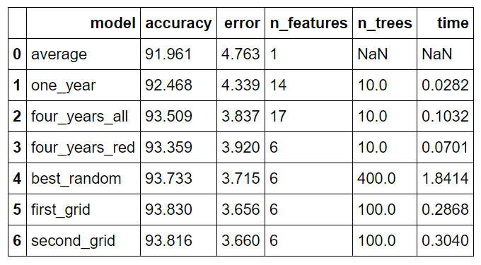Comparison of All Models

Model is the (very unimaginative) names for the models, accuracy is the percentage accuracy, error is the average absolute error in degrees, n_features is the number of features in the dataset, n_trees is the number of decision trees in the forest, and time is the training and predicting time in seconds.

The models are as follows:

• average: original baseline computed by predicting historical average max temperature for each day in test set
• one_year: model trained using a single year of data
• four_years_all: model trained using 4.5 years of data and expanded features (see Part One for details)
• four_years_red: model trained using 4.5 years of data and subset of most important features
• best_random: best model from random search with cross validation
• first_grid: best model from first grid search with cross validation (selected as the final model)
• second_grid: best model from second grid search

Overall, gathering more data and feature selection reduced the error by 17.69% while hyperparameter further reduced the error by 6.73%.

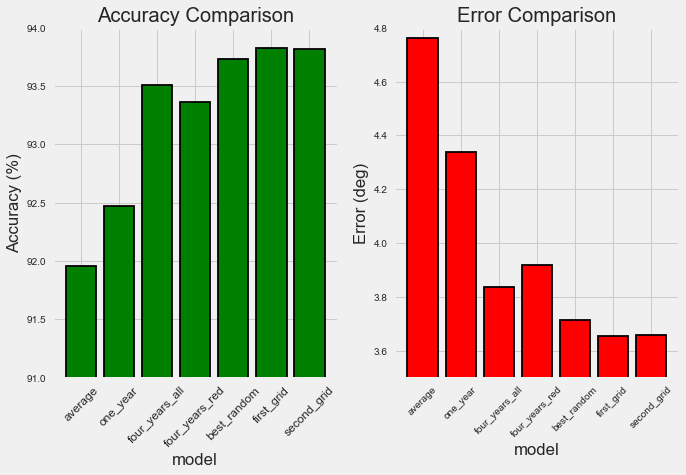Model Comparison (see Notebook for code)

In terms of programmer-hours, gathering data took about 6 hours while hyperparameter tuning took about 3 hours. As with any pursuit in life, there is a point at which pursuing further optimization is not worth the effort and knowing when to stop can be just as important as being able to keep going (sorry for getting all philosophical). Moreover, in any data problem, there is what is called the Bayes error rate, which is the absolute minimum possible error in a problem. Bayes error, also called reproducible error, is a combination of latent variables, the factors affecting a problem which we cannot measure, and inherent noise in any physical process. Creating a perfect model is therefore not possible. Nonetheless, in this example, we were able to significantly improve our model with hyperparameter tuning and we covered numerous machine learning topics which are broadly applicable.

Training Visualizations

To further analyze the process of hyperparameter optimization, we can change one setting at a time and see the effect on the model performance (essentially conducting a controlled experiment). For example, we can create a grid with a range of number of trees, perform grid search CV, and then plot the results. Plotting the training and testing error and the training time will allow us to inspect how changing one hyperparameter impacts the model.

First we can look at the effect of changing the number of trees in the forest. (see notebook for training and plotting code)

Number of Trees Training Curves

As the number of trees increases, our error decreases up to a point. There is not much benefit in accuracy to increasing the number of trees beyond 20 (our final model had 100) and the training time rises consistently.

We can also examine curves for the number of features to split a node:

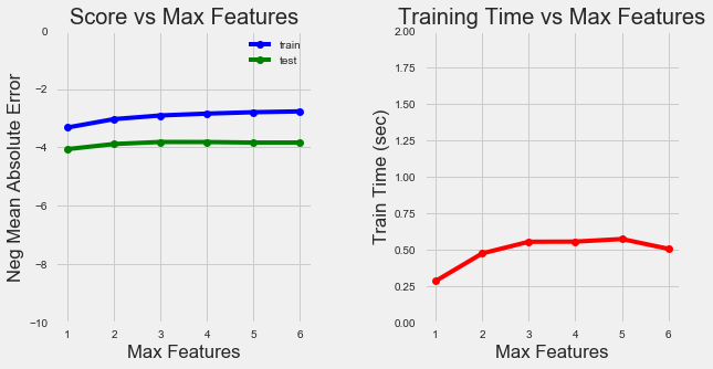Number of Features Training Curves

As we increase the number of features retained, the model accuracy increases as expected. The training time also increases although not significantly.

Together with the quantitative stats, these visuals can give us a good idea of the trade-offs we make with different combinations of hyperparameters. Although there is usually no way to know ahead of time what settings will work the best, this example has demonstrated the simple tools in Python that allow us to optimize our machine learning model.

As always, I welcome feedback and constructive criticism. I can be reached at wjk68@case.edu