Getting the most out of a machine learning model

How best to describe a Kaggle contest? It’s a machine learning education disguised as a competition! Although there are valid criticisms of Kaggle, overall, it’s a great community that provides interesting problems, thousands of data scientists willing to share their knowledge, and an ideal environment for exploring new ideas. As evidence of this, I never would have learned about the Gradient Boosting Machine, or, one of the topics of this article, automated model optimization, were it not for the Kaggle Home Credit contest.

In this article, part three of a series (Part One: Getting Started and Part Two: Improving) documenting my work for this contest, we will focus on a crucial aspect of the machine learning pipeline: model optimization through hyperparameter tuning. In the second article, we decided on the Gradient Boosting Machine as our model of choice, and now we have to get the most out of it through optimization. We’ll do this primarily with two methods: random search and automated tuning with Bayesian optimization.

All the work presented here is available to run on Kaggle in the following notebooks. The article itself will highlight the key ideas but the code details are all in the notebooks (which are free to run with nothing to install!)

1. Random and Grid Search
2. Automated Hyperparameter tuning
3. Tuning Results

For this article we will skip the background, so if at any time you feel lost, I encourage you to go to the previous articles and notebooks. All of the notebooks can be run on Kaggle without the need to download anything, so I highly recommend checking them out or competing!

Recap

In the first part of this series, we got familiar with the dataset, performed exploratory data analysis, tried our hand at feature engineering, and built a few baseline models. Our public leaderboard score from this round was 0.678 (which at the moment would place us lower than 4000 on the leaderboard).

Part two involved in-depth manual feature engineering, followed by feature selection and more modeling. Using the expanded (and then contracted) set of features, we ended up with a score of 0.779, quite an improvement from the baseline, but not quite in the top 50% of competitors. In this article, we will once again better our score and move up 1000 places on the leaderboard.

Machine Learning Optimization

Optimization in the context of machine learning means finding the set of model hyperparameter values that yield the highest cross validation score for a given dataset. Model hyperparameters, in contrast to model parameters that are learned during training, are set by the data scientist before training. The number of layers in a deep neural network is a model hyperparameter while the splits in a decision tree are model parameters. I like to think of model hyperparameters as settings that we need to tune for a dataset: the ideal combination of values is different for every problem!

A machine learning model has to be tuned like a radio — if anyone remembers what a radio was!

There are a handful of ways to tune a machine learning model:

1. Manual: select hyperparameters with intuition/experience/guessing, train the model with the values, and find the validation score Repeat process until you run out of patience or are satisfied with the results.
2. Grid Search: set up a hyperparameter grid and for each combination of values, train a model and find the validation score. In this approach, every combination of hyperparameter values is tried which is very inefficient!
3. Random search: set up a hyperparameter grid and select random combinations of values to train the model and find the validation score. The number of search iterations is based on time/resources.
4. Automated Hyperparameter Tuning: use methods such as gradient descent, Bayesian Optimization, or evolutionary algorithms to conduct a guided search for the best hyperparameters. These methods use the previous results to choose the next hyperparameter values in an informed search compared to random or grid which are uninformed methods.

These are presented in order of increasing efficiency, with manual search taking the most time (and often yielding the poorest results) and automated methods converging on the best values the quickest, although, as with many topics in machine learning, this is not always the case! As shown in this great paper, random search does surprisingly well (which we’ll see shortly).

(There are also other hyperparameter tuning methods such as evolutionary and gradient-based. There are constantly better methods being developed, so make sure to stay up to date on the current best practice!)

In the second part of this series, we decided to use the Gradient Boosting Machine (GBM) model because of its superior performance on structured data with many features. The GBM is extremely powerful (yet easy to implement in Python), but it has dozens of hyperparameters that significantly affect performance and which must be optimized for a problem. If you want to feel overwhelmed, check out the documentation on the LightGBM library:

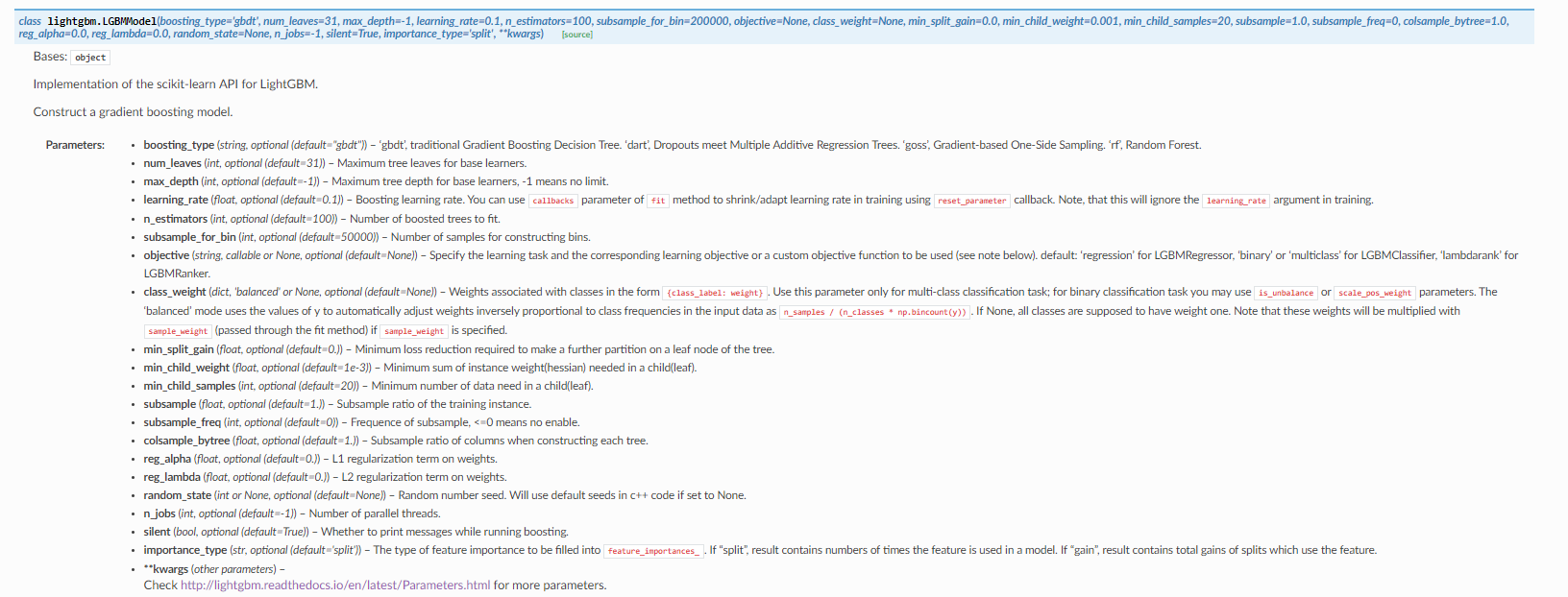LightGBM Documentation

I don’t think there is anyone in the world who can look at all of these and pick the best values! Therefore, we need to implement one of the four methods for choosing the hyperparameters.

For this problem, I didn’t even try manual tuning, both because this was my first time working with the GBM and because I didn’t want to waste any time. e’ll skip straight to random search and automated techniques using Bayesian optimization.

Implementing Grid and Random Search

In the first notebook, we go through an implementation of grid and random search covering the four parts of an optimization problem:

1. Objective function: a function that takes in hyperparameters and returns a score we are trying to minimize or maximize
2. Domain: the set of hyperparameter values over which we want to search.
3. Algorithm: method for selecting the next set of hyperparameters to evaluate in the objective function.
4. Results history: data structure containing each set of hyperparameters and the resulting score from the objective function.

These four parts also form the basis of Bayesian optimization, so laying them out here will help when it comes to that implementation. For the code details, refer to the notebooks, but here we’ll briefly touch on each concept.

Objective Function

The objective function takes in a set of inputs and returns a score that we want to maximize. In this case, the inputs are the model hyperparameters, and the score is the 5-fold cross validation ROC AUC on the training data. The objective function in pseudo-code is:

def objective(hyperparameters):
    """Returns validation score from hyperparameters"""

    model = Classifier(hyperparameters)

validation_loss = cross_validation(model, training_data,
                                       nfolds = 5)

return validation_loss

The goal of hyperparameter optimization is to find the hyperparameters that return the best value when passed into the objective function. That seems pretty simple, but the problem is evaluating the objective function is very expensive in terms of time and computational resources. We cannot try every combination of hyperparameter values because we have a limited amount of time, hence the need for random search and automated methods.

Domain

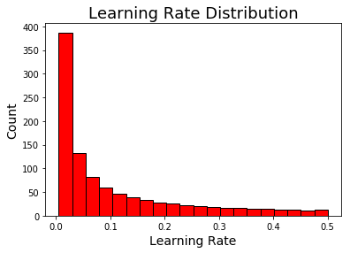
The domain is the set of values over which we search. For this problem with a GBM, the domain is as follows:

We can visualize two of these distributions, the learning rate, which is logarithmic normal, and the number of leaves which is uniform normal:

# Algorithm

Although we don’t generally think of them as such, both grid and random search are algorithms. In the case of grid search, we input the domain and the algorithm selects the next value for each hyperparameter in an ordered sequence. The only requirement of grid search is that it tries every combination in a grid once (and only once). For random search, we input the domain and each time the algorithm gives us a random combination of hyperparameter values to try. There are no requirements for random search other than that the next values are selected at random.

Random search can be implemented as in the following:

import random

_# Randomly sample from dictionary of hyperparameters_
random_params = {k: random.sample(v, 1)[0] for k, v **in**
                    param_grid.items()}

**{'boosting_type': 'goss',
 'colsample_bytree': 0.8222222222222222,
 'is_unbalance': False,
 'learning_rate': 0.027778881111994384,
 'min_child_samples': 175,
 'num_leaves': 88,
 'reg_alpha': 0.8979591836734693,
 'reg_lambda': 0.6122448979591836,
 'subsample': 1.0,
 'subsample_for_bin': 220000}**

This is in effect a very simple algorithm!

Results History

The results history is a data structure that contains the hyperparameter combinations and the resulting score on the objective function. When we get to Bayesian Optimization, the model actually uses the past results to decide on the next hyperparmeters to evaluate. Random and grid search are uninformed methods that do not use the past history, but we still need the history so we can find out which hyperparameters worked the best!

In this case, the results history is simply a dataframe.

# Bayesian Hyperparameter Optimization

Automated hyperparameter tuning with bayesian optimization sounds complicated, but in fact it uses the same four parts as random search with the only difference the Algorithm used. For this competition, I used the Hyperopt library and the Tree Parzen Estimator (TPE) algorithm with the work shown in this notebook. For a conceptual explanation, refer to this article, and for an implementation in Python, check out the notebook or this article.

The basic concept of Bayesian optimization is that it uses the previous evaluation results to reason about which hyperparameters perform better and uses this reasoning to choose the next values. Hence, this method should spend fewer iterations evaluating the objective function with poorer values. Theoretically, Bayesian optimization can converge on the ideal values in fewer iterations than random search (although random search can still get lucky)! The aspirations of Bayesian optimization are:

1. To find better hyperparameter values as measured by performance
2. Use fewer iterations for optimization than grid or random search

This is a powerful method that promises to deliver great results. The question is, does the evidence in practice show this to be the case? To answer that, we turn to the final notebook, a deep dive into the model tuning results!

Hyperparameter Optimization Results

After the hard work of implementing random search and Bayesian optimization, the third notebook is a fun and revealing exploration of the results. There are over 35 plots, so if you like visuals, then check it out.

Although I was trying to do the whole competition on Kaggle, for these searches, I did 500 iterations of random search and 400 of Bayesian optimization which took about 5 days each on a computer with 64 GB of RAM (thanks to Amazon AWS). All the results are available, but you’ll need some serious hardware to redo the experiments!

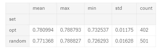
First off: which method did better? The image below summarizes the results from 501 iterations of random search and 402 of Bayesian optimization (called opt in the dataframe):

Random Search and Bayesian Optimization ( opt) results

Going by max score, random search does slightly better but if we measure by average score, bayesian optimization wins.

The good news is this is almost exactly what we expect: random search can happen upon a great set of values because it thoroughly explores the search space, but Bayesian optimization will “focus” on the highest scoring hyperparameter values by reasoning from previous results. Let’s take a look at a very revealing plot, the value of the cross validation score versus the number of iterations:

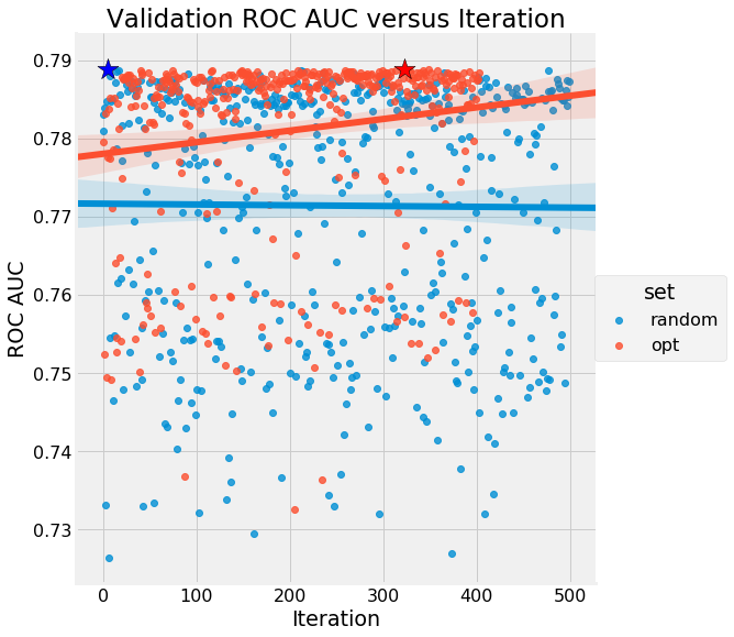We see absolutely no trend for random search, while Bayesian Optimization (again shown by opt ) improves over the trials. If you can understand this graph, then you can see the benefits of both methods: random search explores the search domain but Bayesian optimization gets better over time. We can also see that Bayesian optimization appears to reach a plateau, indicating diminishing returns to further trials.

Second major question: what were the best hyperparameter values? Below are the optimal results from Bayesian optimization:

**boosting_type             gbdt
colsample_bytree      0.614938
is_unbalance              True
learning_rate        0.0126347
metric                     auc
min_child_samples          390
n_estimators              1327
num_leaves                 106
reg_alpha             0.512999
reg_lambda            0.382688
subsample             0.717756
subsample_for_bin        80000
verbose                      1
iteration                  323
score                 0.788793**

We can use these results to build a model and submit predictions to the competition, or they can be used to inform further searches by allowing us to define a concentrated search space around the best values.

Hyperparameter Plots

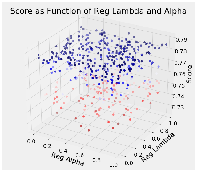
One interesting aspect to consider is the values tried by each search method for each hyperparameter. The plots below show kernel density estimate (KDE) functions for each of the search methods as well as the sampling distribution (the hyperparameter grid). The dashed vertical lines indicate the optimal value found for each method. First is the learning rate:

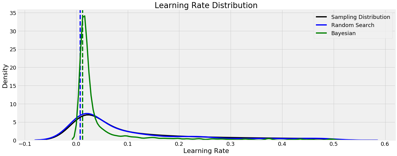Even though the learning rate distribution stretched over several orders of magnitude, both methods found optimal values quite low in the domain. We can use this knowledge to inform further hyperparameter searches by concentrating our search in this region. In most cases, a lower learning rate increases the cross validation performance but at the cost of increased run-time, which is a trade-off we have to make.

Let’s look at some other graphs. For most of the hyperparameters, the optimal values from both methods are fairly close, but not for colsample_bytree :

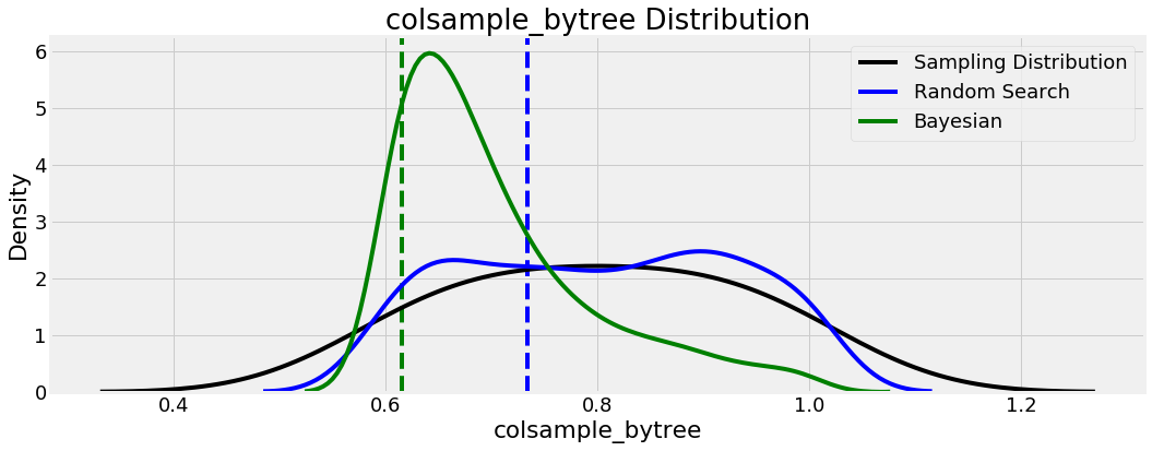This refers to the fraction of columns used when building each tree in the GBM, and random search found the optimal value was higher than Bayesian optimization. Again, these results can be used for further searches, as we see that the Bayesian method tended to concentrate on values around 0.65.

We’ll show two more plots from this analysis because they are fairly interesting, involving two regularization parameters:

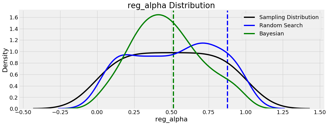
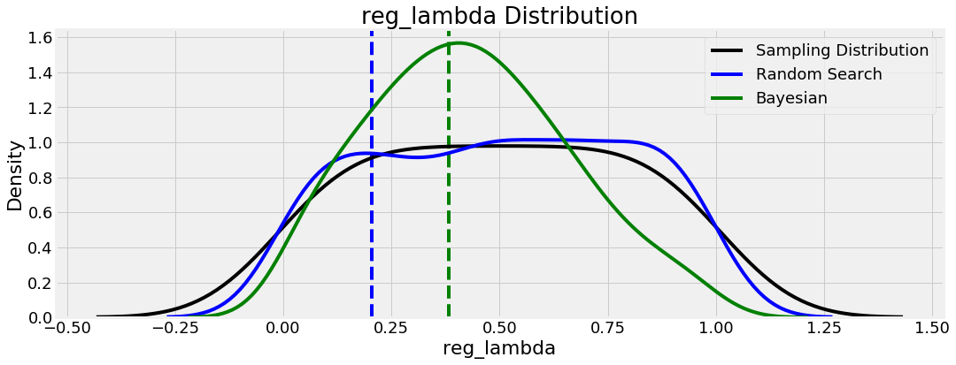What’s noteworthy here is that these two hyperparameters appear to be complements of one another: if one regularization value is high, then we want the other to be low and vice versa. Maybe this helps the model achieve a balance between bias/variance, the most common issue in machine learning.

Hyperparameters versus Iteration

While random search does not change the distribution of values over the search, Bayesian optimization does, by concentrating on where it thinks the best values are in the search domain. We can see this by graphing the hyperparameter values against the iteration:

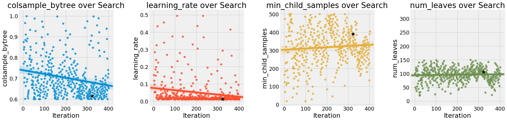
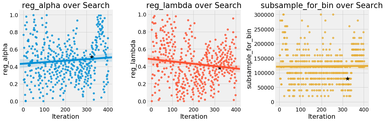The hyperparameters with the clearest trend are colsample_bytree and learning_rate which both continue downward over the trials. The reg_lambda and reg_alpha are diverging, which confirms our earlier hypothesis that we should decrease one of these while increasing the other.

We want to be careful about placing too much value in these results, because the Bayesian optimization might have found a local minimum of the cross validation loss that it is exploiting. The trends here are pretty small, but it’s encouraging that the best value was found close to the end of the search indicating cross validation scores were continuing to improve.

Hyperparameter versus Cross Validation Score

These next plots show the value of a single hyperparameter versus the score. We want to avoid placing too much emphasis on these graphs because we are not changing one hyperparameter at a time and there can be complex interactions between multiple hyperparameters. A truly accurate graph would be 10-dimensional and show the values of all hyperparameters and the resulting score. If we could understand a 10-dimensional graph, then we might be able to figure out the optimal combination of hyperparameters!

Here the random search is in blue and the Bayesian in green:

The only clear distinction is that the score decreases as the learning rate increases. We cannot say whether that is due to the learning rate itself, or some other factor (we will look at the interplay between the learning rate and the number of estimators shortly).

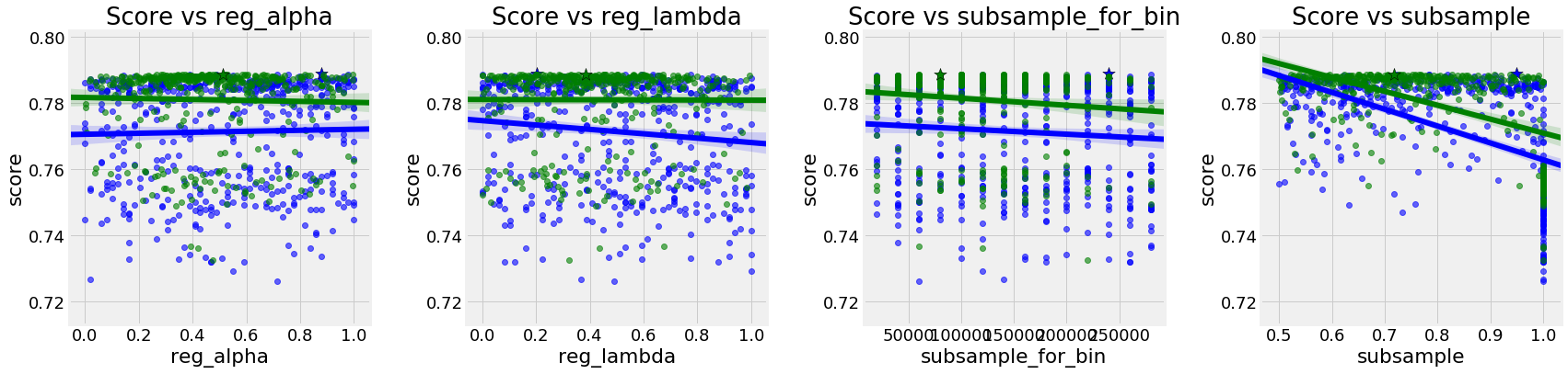There are not any strong trends here. The score versus subsample is a little off because boosting_type = 'goss' cannot use subsample (it must be set equal to 1.0). While we can’t look at all 10 hyperparameters at one time, we can view two at once if we turn to 3D plots!

3D Plots

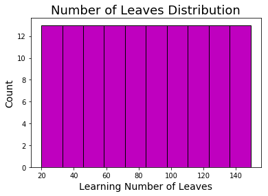
To try and examine the simultaneous effects of hyperparameters, we can make 3D plots with 2 hyperparameters and the score. A truly accurate plot would be 10-D (one for each hyperparameter) but in this case we will stick to 3 dimensions. (See the code for details, 3D plotting in Python is surprisingly straightforward). First we can show the reg_alpha and reg_lambda , the regularization hyperparameters versus the score (for Bayesian opt):

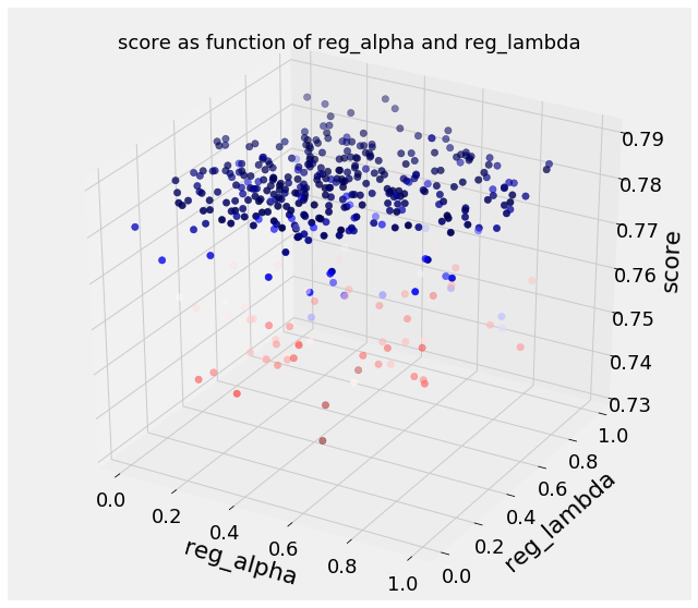It’s a little hard to make sense, but if we remember the best scores occurred around 0.5 for reg_alpha and 0.4 for reg_lambda , we can see generally better scores in this region.

Next is the learning_rate and n_estimators (number of decision trees trained in the ensemble). While the learning rate was a hyperparameter in the grid, the number of decision trees (also called the number of boosting rounds) was found by early stopping with 5-fold cross validation:

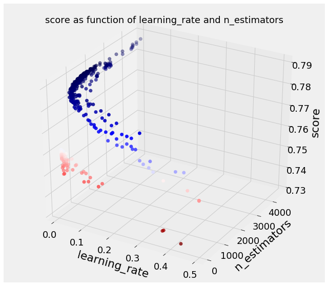This time there is a clear trend: a lower learning rate and higher number of estimators increases the score. The relationship is expected because a lower learning rate means the contribution of each tree is reduced which necessitates training more trees. The expanded number of trees increases the model’s capacity to fit the training data (while also increasing the time to run). Moreover, as long as we use early stopping with enough folds, we don’t have to be concerned about overfitting with more trees. It’s nice when the results agree with our understanding (_although we probably learn more when they don’t agree!_)

Correlation Heatmaps

For the final plot, I wanted to show the correlations between each hyperparameter and each other and the score. These plots can’t prove causation, but they can tell us which variables are correlated:

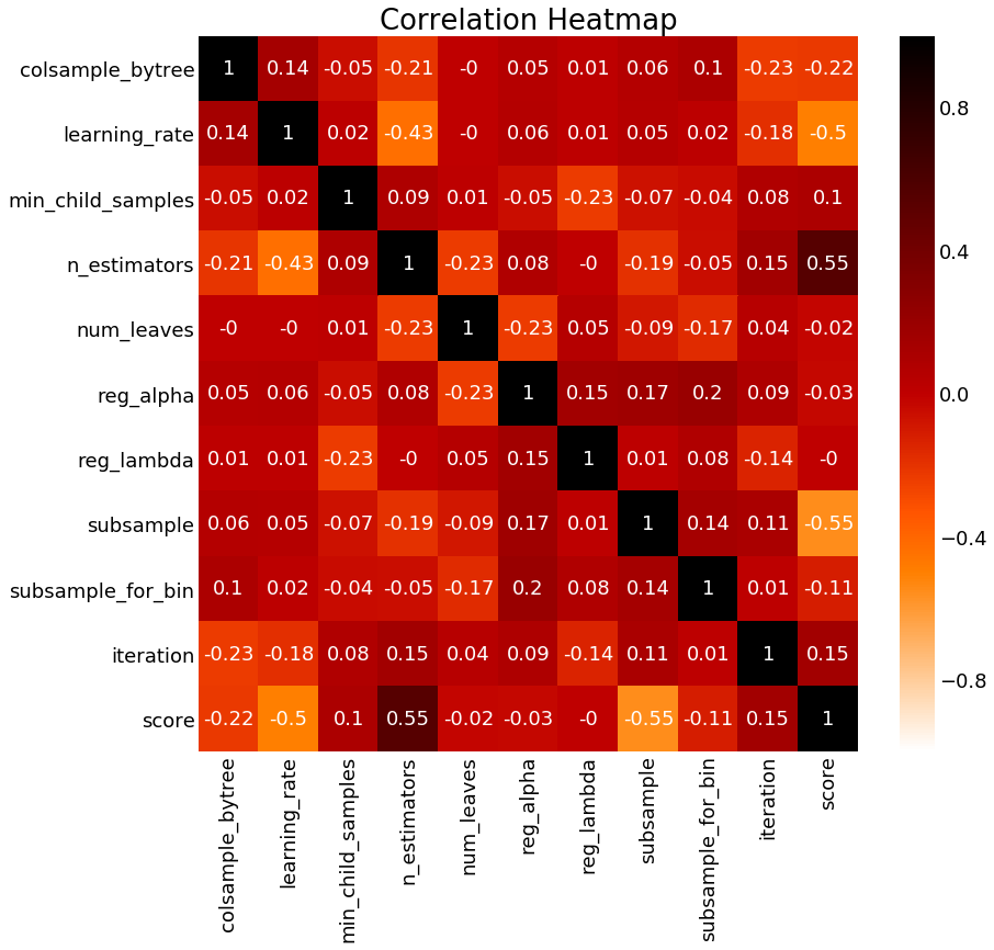Correlation Heatmap for Bayesian Optimization

We already found most of the information from the graphs, but we can see the negative correlation between the learning rate and the score, and the positive correlation between the number of estimators and the score.

Testing Optimal Hyperparameters

The final step of the exploration was to implement both the random search best hyperparameters and the Bayesian optimization best hyperparameters on a full dataset (the dataset comes from this kernel and I would like to thank the author for making it public). We train the model, make predictions on the testing set, and finally upload to the competition to see how we do on the public leaderboard. After all the hard work, do the results hold up?

• Random search results scored 0.790
• Bayesian optimization results scored 0.791

If we go by best score on the public leaderboard, Bayesian Optimization wins! However, the public leaderboard is based only on 10% of the test data, so it’s possible this is a result of overfitting to this particular subset of the testing data. Overall, I would say the complete results — including cross validation and public leaderboard — suggest that both methods produce similar outcomes when run for enough iterations. All we can say for sure is that either method is better than hand-tuning! Our final model is enough to move us 1000 places up the leaderboard compared to our previous work.

Finally, to end with one more plot, we can take a look at the feature importances from the trained GBM:

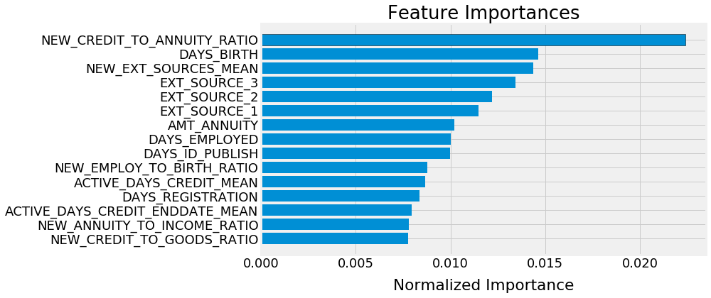
NEW_CREDIT_TO_ANNUITY_RATIO and NEW_EXT_SOURCES_MEAN were features derived by the data science community on Kaggle and not in the original data. It’s reassuring to see these so high up in the importance because it shows the value of feature engineering.

Conclusions and Next Steps

The major takeaways from this work are:

• Random search and automated hyperparameter tuning using Bayesian optimization are effective methods for model tuning
• Bayesian optimization tends to “concentrate” on higher scoring values while random search better explores the possibilities
• When given enough iterations, both methods produce similar results in terms of cross validation and test scores
• Optimizing the hyperparameters has a significant effect on performance, comparable to feature engineering for this problem

Where to go from here? Well, there are always plenty of other methods to try such as automated feature engineering or treating the problem as a time-series. I’ve already done a notebook on automated feature engineering so that will probably be where my focus will turn next. We can also try other models or even journey into the realm of deep learning!

I’m open to suggestions, so let me know on Kaggle or on Twitter. Thanks for reading, and if you want to check out any of my other work on this problem, here are the complete set of notebooks:

• A Gentle Introduction
• Manual Feature Engineering Part One
• Manual Feature Engineering Part Two
• Introduction to Automated Feature Engineering
• Advanced Automated Feature Engineering
• Feature Selection
• Intro to Model Tuning: Grid and Random Search
• Automated Model Tuning
• Model Tuning Results

There should be enough content there to keep anyone busy for a little bit. Now it’s off to do more learning/exploration for the next post! The best part about data science is that you’re constantly on the move, looking for the next technique to conquer. Whenever I find out what that is, I’ll be sure to share it!

As always, I welcome feedback and constructive criticism. I can be reached on Twitter @koehrsen_will.