
Machine Learning Kaggle Competition Part Two Improving

Feature engineering, feature selection, and model evaluation
Like most problems in life, there are several potential approaches to a Kaggle competition:
- Lock yourself away from the outside world and work in isolation
I recommend against the “lone genius” path, not only because it’s exceedingly lonely, but also because you will miss out on the most important part of a Kaggle competition: learning from other data scientists. If you work by yourself, you end up relying on the same old methods while the rest of the world adopts more efficient and accurate techniques.
As a concrete example, I recently have been dependent on the random forest model, automatically applying it to any supervised machine learning task. This competition finally made me realize that although the random forest is a decent starting model, everyone else has moved on to the superior gradient boosting machine.
The other extreme approach is also limiting:
- Copy one of the leader’s scripts (called “kernels” on Kaggle), run it, and shoot up the leaderboard without writing a single line of code
I also don’t recommend the “copy and paste” approach, not because I’m against using other’s code (with proper attribution), but because you are still limiting your chances to learn. Instead, what I do recommend is a hybrid approach: read what others have done, understand and even use their code, and build on other’s work with your own ideas. Then, release your code to the public so others can do the same process, expanding the collective knowledge of the community.
In the second part of this series about competing in a Kaggle machine learning competition, we will walk through improving on our initial submission that we developed in the first part.
The major results documented in this article are:
- An increase in ROC AUC from a baseline of 0.678 to 0.779
- Over 1000 places gained on the leaderboard
- Feature engineering to go from 122 features to 1465
- Feature selection to reduce the final number of features to 342
- Decision to use a gradient boosting machine learning model
We will walk through how we achieve these results — covering a number of major ideas in machine learning and building on other’s code where applicable. We’ll focus on three crucial steps of any machine learning project:
- Feature engineering
- Feature selection
- Model evaluation
To get the most out of this post, you’ll want to follow the Python notebooks on Kaggle (which will be linked to as they come up). These notebooks can be run on Kaggle without downloading anything on your computer so there’s little barrier to entry! I’ll hit the major points at a high-level in this article, with the full details in the notebooks.
Brief Recap
If you’re new to the competition, I highly recommend starting with this article and this notebook to get up to speed.
 The Home Credit Default Risk competition on Kaggle is a standard machine learning classification problem. Given a dataset of historical loans, along with clients’ socioeconomic and financial information, our task is to build a model that can predict the probability of a client defaulting on a loan.
In the first part of this series, we went through the basics of the problem, explored the data, tried some feature engineering, and established a baseline model. Using a random forest and only one of the seven data tables, we scored a 0.678 ROC AUC (Receiver Operating Characteristic Area Under the Curve) on the public leaderboard. (The public leaderboard is calculated with only 20% of the test data and the final standings usually change significantly.)
To improve our score, in this article and a series of accompanying notebooks on Kaggle, we will concentrate primarily on feature engineering and then on feature selection. Generally, the largest benefit relative to time invested in a machine learning problem will come in the feature engineering stage. Before we even start trying to build a better model, we need to focus on using all of the data in the most effective manner!
Notes on the Current State of Machine Learning
Much of this article will seem exploratory (or maybe even arbitrary) and I don’t claim to have made the best decisions! There are a lot of knobs to tune in machine learning, and often the only approach is to try out different combinations until we find the one that works best. Machine learning is more empirical than theoretical and relies on testing rather than working from first principles or a set of hard rules.
In a great blog post, Pete Warden explained that machine learning is a little like banging on the side of the TV until it works. This is perfectly acceptable as long as we write down the exact “bangs” we made on the TV and the result each time. Then, we can analyze the choices we made, look for any patterns to influence future decisions, and find which method works the best.
My goal with this series is to get others involved with machine learning, put my methods out there for feedback, and document my work so I can remember what I did for the next time! Any comments or questions, here or on Kaggle, are much appreciated.
Feature Engineering
Feature engineering is the process of creating new features from existing data. The objective is to build useful features that can help our model learn the relationship between the information in a dataset and a given target. In many cases — including this problem — the data is spread across multiple tables. Because a machine learning model must be trained with a single table, feature engineering requires us to summarize all of the data in one table.
This competition has a total of 7 data files. In the first part, we used only a single source of data, the main file with socioeconomic information about each client and characteristics of the loan application. We will call this table app.(For those used to Pandas, a table is just a dataframe).
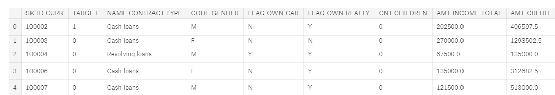 Main training dataframe
We can tell this is the training data because it includes the label, TARGET. A TARGET value of 1 indicates a loan which was not repaid.
The app dataframe is tidy structured data: there is one row for every observation — a client’s application for a loan — with the columns containing the features (also known as the explanatory or predictor variables). Each client’s application — which we will just call a “client” — has a single row in this dataframe identified by the SK_ID_CURR. Because each client has a unique row in this dataframe, it is the parent of all the other tables in the dataset as indicated by this diagram showing how the tables are related:
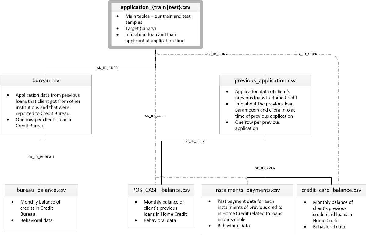 Relationship of data files (Source)
When we make our features, we want to add them to this main dataframe. At the end of feature engineering, each client will still have only a single row, but with many more columns capturing information from the other data tables.
The six other tables contain information about clients’ previous loans, both with Home Credit (the institution running the competition), and other credit agencies. For example, here is the bureau dataframe, containing client’s previous loans at other financial institutions:
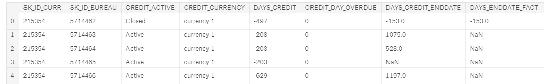 bureau dataframe, a child of app
This dataframe is a child table of the parentapp: for each client (identified by SK_ID_CURR) in the parent, there may be many observations in the child. These rows correspond to multiple previous loans for a single client. The bureau dataframe in turn is the parent of the bureau_balance dataframe where we have monthly information for each previous loan.
Let’s look at an example of creating a new feature from a child dataframe: the count of the number of previous loans for each client at other institutions. Even though I wrote a post about automated feature engineering, for this article we will stick to doing it by hand. The first Kaggle notebook to look at is here: is a comprehensive guide to manual feature engineering.
Calculating this one feature requires grouping (using groupby)the bureau dataframe by the client id, calculating an aggregation statistic (using agg with count) and then merging (using merge) the resulting table with the main dataframe. This means that for each client, we are gathering up all of their previous loans and counting the total number. Here it is in Python:
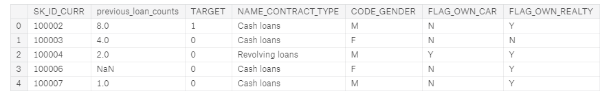 app dataframe with new feature in second column
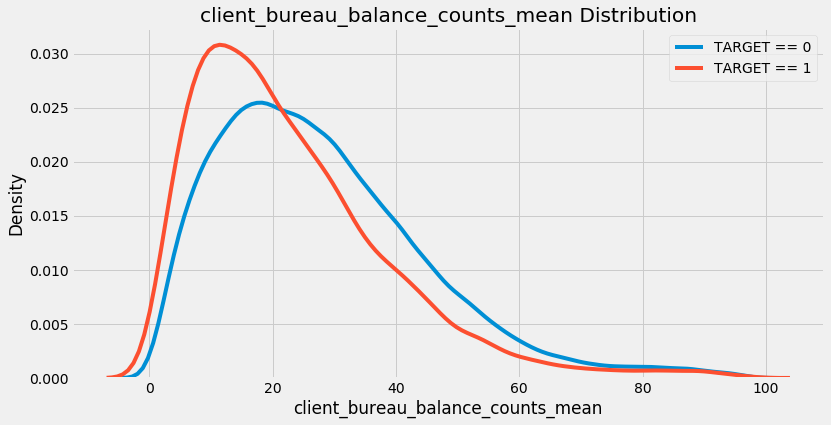
Now our model can use the information of the number of previous loans as a predictor for whether a client will repay a loan. To inspect the new variable, we can make a kernel density estimate (kde) plot. This shows the distribution of a single variable and can be thought of as a smoothed histogram. To see if the distribution of this feature varies based on whether the client repaid her/his loan, we can color the kde by the value of the TARGET:
 There does not appear to be much of a difference in the distribution, although the peak of the
 TARGET==1 distribution is slightly to the left of the TARGET==0 distribution. This could indicate clients who did not repay the loan tend to have had fewer previous loans at other institutions. Based on my extremely limited domain knowledge, this relationship would make sense!
Generally, we do not know whether a feature will be useful in a model until we build the model and test it. Therefore, our approach is to build as many features as possible, and then keep only those that are the most relevant. “Most relevant” does not have a strict definition, but we will see some ways we can try to measure this in the feature selection section.
Now let’s look at capturing information not from a direct child of the app dataframe, but from a child of a child of app! The bureau_balance dataframe contains monthly information about each previous loan. This is a child of the bureau dataframe so to get this information into the main dataframe, we will have to do two groupbys and aggregates: first by the loan id (SK_ID_BUREAU) and then by the client id.
As an example, if we want to calculate for each client the average of the max number of MONTHS_BALANCE for each previous loan in the bureau_balance dataframe, we can do this:
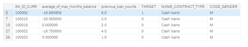 app dataframe with new feature in second column
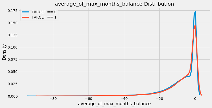 Distribution of new feature
This was a lot of code for a single feature, and you can easily imagine that the manual feature engineering process gets tedious after a few features! That’s why we want to write functions that take these individual steps and repeat them for us on each dataframe.
Instead of repeating code over and over, we put it into a function — called refactoring — and then call the function every time we want to perform the same operation. Writing functions saves us time and allows for more reproducible workflows because it will execute the same actions in exactly the same way every time.
Below is a function based on the above steps that can be used on any child dataframe to compute aggregation statistics on the numeric columns. It first groups the columns by a grouping variable (such as the client id), calculates the mean, max, min, sum of each of these columns, renames the columns, and returns the resulting dataframe. We can then merge this dataframe with the main app data.
(This function draws heavily on this kernel from olivier on Kaggle).
(Half of the lines of code for this function is documentation. Writing proper docstrings is crucial not only for others to understand our code, but so we can understand our own code when we come back to it!)
To see this in action, refer to the notebook, but clearly we can see this will save us a lot of work, especially with 6 children dataframes to process.
This function handles the numeric variables, but that still leaves the categorical variables. Categorical variables, often represented as strings, can only take on a limited number of values (in contrast to continuous variables which can be any numeric value). Machine learning models cannot handle string data types, so we have to find a way to capture the information in these variables in a numeric form.
As an example of a categorical variable, the bureau table has a column called CREDIT_ACTIVE that has the status of each previous loan:
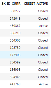 Two columns of the bureau dataframe showing a categorical variable (CREDIT_ACTIVE)
We can represent this data in a numeric form by counting the number of each type of loan that each client has had. Moreover, we can calculate the normalized count of each loan type by dividing the count for one particular type of loan by the total count. We end up with this:
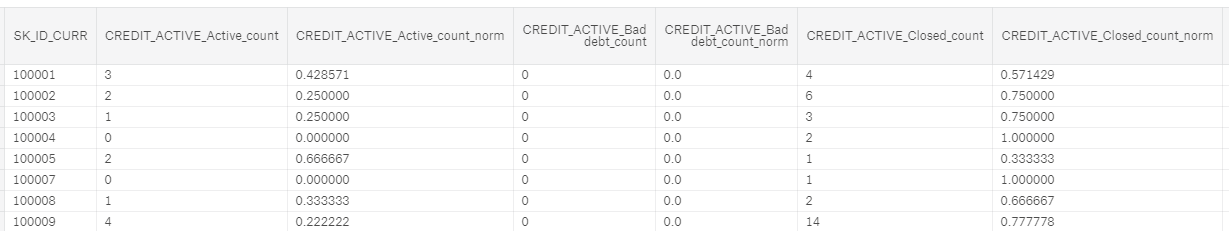 Categorical CREDIT_ACTIVE features after processing
Now these categorical features can be passed into a machine learning model. The idea is that we capture not only the number of each type of previous loan, but also the relative frequency of that type of loan. As before, we don’t actually know whether these new features will be useful and the only way to say for sure is to make the features and then test them in a model!
Rather than doing this by hand for every child dataframe, we again can write a function to calculate the counts of categorical variables for us. Initially, I developed a really complicated method for doing this involving pivot tables and all sorts of aggregations, but then I saw other code where someone had done the same thing in about two lines using one-hot encoding. I promptly discarded my hours of work and used this version of the function instead!
This function once again saves us massive amounts of time and allows us to apply the same exact steps to every dataframe.
Once we write these two functions, we use them to pull all the data from the seven separate files into one single training (and one testing dataframe). If you want to see this implemented, you can look at the first and second manual engineering notebooks. Here’s a sample of the final data:
 Using information from all seven tables, we end up with a grand total of 1465 features! (From an original 122).
How do we know if any of these features are helpful? One method is to calculate the Pearson correlation coefficient between the variables and the TARGET. This is a relatively crude measure of importance, but it can serve as an approximation of which variables are related to a client’s ability to repay a loan. Below are the most correlated variables with the TARGET:
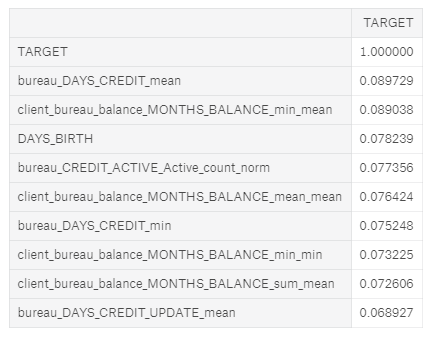
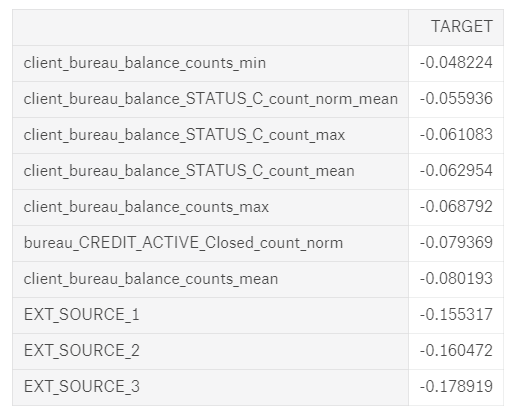 Most Positive (left) and Negative (right) correlated variables with the TARGET
The EXT_SOURCE_ variables were from the original features, but some of the variables we created are among the top correlations. However, we want to avoid reading too much into these numbers. Anytime we make a ton of features, we can run into the multiple comparisons problem: the more comparisons we make — in this case correlations with the target — the more likely some of them are to be large due to random noise. With correlations this small, we need to be especially careful when interpreting the numbers.
The most negatively correlated variable we made, client_bureau_balance_counts_mean, represents the average for each client of the count of the number of times a loan appeared in the bureau_balance data. In other words, it is the average number of monthly records per previous loan for each client. The kde plot is below:
 Now that we have 1465 features, we run into the problem of too many features! More menacingly, this is known as the curse of dimensionality, and it is addressed through the crucial step of feature selection.
Feature Selection
Too many features can slow down training, make a model less interpretable, and, most critically, reduce the model’s generalization performance on the test set. When we have irrelevant features, these drown out the important variables and as the number of features increases, the number of data points needed for the model to learn the relationship between the data and the target grows exponentially (curse of dimensionality explained).
After going to all the work of making these features, we now have to select only those that are “most important” or equivalently, discard those that are irrelevant.
The next notebook to go through is here: a guide to feature selection which is fairly comprehensive although it still does not cover every possible method!
There are many ways to reduce the number of features, and here we will go through three methods:
- Removing collinear variables
- Removing variables with many missing values
- Using feature importances to keep only “important” variables
Remove Collinear Variables
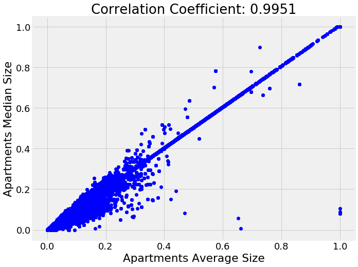
Collinear variables are variables that are highly correlated with one another. These variables are redundant in the sense that we only need to keep one out of each pair of collinear features in order to retain most of the information in both. The definition of highly correlated can vary and this is another of those numbers where there are no set rules! As an example of collinear variables, here is a plot of the median apartment size vs average apartment size:
 To identify highly correlated variables, we can calculate the correlation of every variable in the data with every other variable (this is quite a computationally expensive process)! Then we select the upper triangle of the correlation matrix and remove one variable from every pair of highly correlated variables based on a threshold. This is implemented in code below:
(This code is adapted from this blog post.)
In this implementation, I use a correlation coefficient threshold of 0.9 to remove collinear variables. So, for each pair of features with a correlation greater than 0.9, we remove one of the pair of features. Out of 1465 total features, this removes 583, indicating many of the variables we created were redundant.
Remove Missing Columns
Of all the feature selection methods, this seems the most simple: just eliminate any columns above a certain percentage of missing values. However, even this operation brings in another choice to make, the threshold percentage of missing values for removing a column.
Moreover, some models, such as the Gradient Boosting Machine in LightGBM, can handle missing values with no imputation and then we might not want to remove any columns at all! However, because we’ll eventually test several models requiring missing values to be imputed, we’ll remove any columns with more than 75% missing values in either the training or testing set.
This threshold is not based on any theory or rule of thumb, rather it’s based on trying several options and seeing which worked best in practice. The most important point to remember when making these choices is that they don’t have to be made once and then forgotten. They can be revisited again later if the model is not performing as well as expected. Just make sure to record the steps you took and the performance metrics so you can see which works best!
Dropping columns with more than 75% missing values removes 19 columns from the data, leaving us with 863 features.
Feature Selection Using Feature Importances
The last method we will use to select features is based on the results from a machine learning model. With decision tree based classifiers, such as ensembles of decision trees (random forests, extra trees, gradient boosting machines), we can extract and use a metric called the feature importances.
The technical details of this is complicated (it has to do with the reduction in impurity from including the feature in the model), but we can use the relative importances to determine which features are the most helpful to a model. We can also use the feature importances to identify and remove the least helpful features to the model, including any with 0 importance.
To find the feature importances, we will use a gradient boosting machine (GBM) from the LightGBM library. The model is trained using early stopping with two training iterations and the feature importances are averaged across the training runs to reduce the variance.
Running this on the features identifies 308 features with 0.0 importance.
Removing features with 0 importance is a pretty safe choice because these are features that are literally never used for splitting a node in any of the decision trees. Therefore, removing these features will have no impact on the model results (at least for this particular model).
This isn’t necessary for feature selection, but because we have the feature importances, we can see which are the most relevant. To try and get an idea of what the model considers to make a prediction, we can visualize the top 15 most important features:
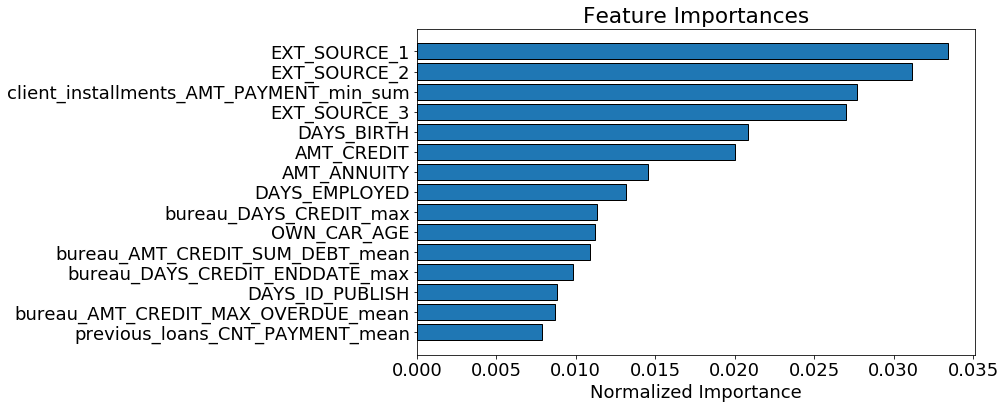 Top 15 most important features
We see that a number of the features we built made it into the top 15 which should give us some confidence that all our hard work was worthwhile! One of our features even made it into the top 5. This feature, client_installments_AMT_PAYMENT_min_sum represents the sum of the minimum installment payment for each client of their previous loans at Home Credit. That is, for each client,it is the sum of all the minimum payments they made on each of their previous loans.
The feature importance don’t tell us whether a lower value of this variable corresponds to lower rates of default, it only lets us know that this feature is useful for making splits of decision trees nodes. Feature importances are useful, but they do not offer a completely clear interpretation of the model!
After removing the 0 importance features, we have 536 features and another choice to make. If we think we still have too many features, we can start removing features that have a minimal amount of importance. In this case, I continued with feature selection because I wanted to test models besides the gbm that do not do as well with a large number of features.
The final feature selection step we do is to retain only the features needed to account for 95% of the importance. According to the gradient boosting machine, 342 features are enough to cover 95% of the importance. The following plot shows the cumulative importance vs the number of features.
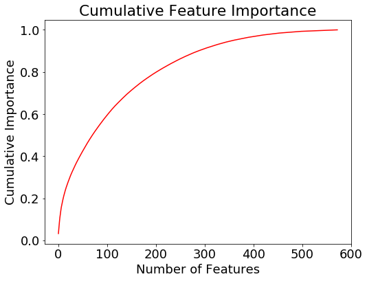 Cumulative feature importance from the gradient boosting machine
There are a number of other dimensionality reduction techniques we can use, such as principal components analysis (PCA). This method is effective at reducing the number of dimensions, but it also transforms the features to a lower-dimension feature space where they have no physical representation, meaning that PCA features cannot be interpreted. Moreover, PCA assumes the data is normally distributed, which might not be a valid assumption for human-generated data. In the notebook I show how to use pca, but don’t actually apply it to the data.
We can however use pca for visualizations. If we graph the first two principal components colored by the value of the TARGET , we get the following image:
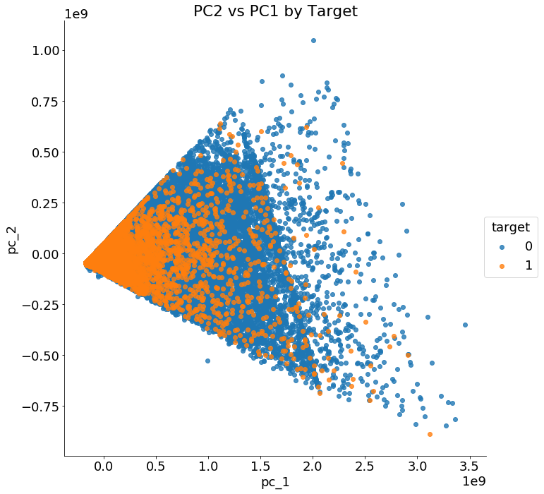 First two principal components of the data
The two classes are not cleanly separated with only two principal components and clearly we need more than two features to identify customers who will repay a loan versus those who will not.
Before moving on, we should record the feature selection steps we took so we remember them for future use:
- Remove collinear variables with a correlation coefficient greater than 0.9: 583 features removed
- Remove columns with more than 75% missing values: 19 features removed
- Remove 0.0 importance features according to a GBM: 308 features removed
- Keep only features needed for 95% of feature importance: 193 features removed
The final dataset has 342 features.
If it seems like there are a few arbitrary choices made during feature selection, that’s because there were! At a later point, we might want to revisit some of these choices if we are not happy with our performance. Fortunately, because we wrote functions and documented our decisions, we can easily change some of the parameters and then reassess performance.
Model Selection
Generally, at this point in a machine learning problem, we would move on to evaluating a number of models. No model is better than all others at every task (the “no free lunch theorem”), and so we need to try out a range of models to determine which one to use. However, in recent years, one model has become increasingly successful for problems with medium-sized structured data: the gradient boosting machine. (There are a number of reasons why this model works so well, and for a comprehensive guide, this Master’s Thesis is a great read.)
Model selection is one area where I relied heavily on the work of others. As mentioned at the beginning of the post, prior to this competition, my go-to model was the random forest. Very early on in this competition though, it was clear from reading the notebooks of others that I would need to implement some version of the gradient boosting machine in order to compete. Nearly every submission at the top of the leaderboard on Kaggle uses some variation (or multiple versions) of the Gradient Boosting Machine. (Some of the libraries you might see used are LightGBM, CatBoost, and XGBoost.)
Over the past few weeks, I have read through a number of kernels (see here and here) and now feel pretty confident deploying the Gradient Boosting Machine using the LightGBM library (Scikit-Learn does have a GBM, but its not as efficient or as accurate as other libraries). Nonetheless, mostly for curiosity’s sake, I wanted to try several other methods to see just how much is gained from the GBM. The code for this testing can be found on Kaggle here.
This isn’t entirely a fair comparison because I was using mostly the default hyperparameters in Scikit-Learn, but it should give us a first approximation of the capabilities of several different models. Using the dataset after applying all of the feature engineering and the feature selection, below are the modeling results with the public leaderboard scores. All of the models except for the LightGBM are built in Scikit-Learn:
- Logistic Regression = 0.768
- Random Forest with 1000 trees = 0.708
- Extra Trees with 1000 trees = 0.725
- Gradient Boosting Machine in Scikit-Learn with 1000 trees = 0.761
- Gradient Boosting Machine in LightGBM with 1000 trees = 0.779
- Average of all Models = 0.771
It turns out everyone else was right: the gradient boosting machine is the way to go. It returns the best performance out of the box and has a number of hyperparameters that we can adjust for even better scores. That does not mean we should forget about other models, because sometimes adding the predictions of multiple models together (called ensembling) can perform better than a single model by itself. In fact, many winners of Kaggle competitions used some form of ensembling in their final models.
We didn’t spend too much time here on the models, but that is where our focus will shift in the next notebooks and articles. Next we can work on optimizing the best model, the gradient boosting machine, using hyperparameter optimization. We may also look at averaging models together or even stacking multiple models to make predictions. We might even go back and redo feature engineering! The most important points are that we need to keep experimenting to find what works best, and we can read what others have done to try and build on their work.
Conclusions
Important character traits of being a data scientist are curiosity and admitting you don’t know everything! From my place on the leaderboard, I clearly don’t know the best approach to this problem, but I’m willing to keep trying different things and learn from others. Kaggle competitions are just toy problems, but that doesn’t prevent us from using them to learn and practice concepts to apply to real projects.
In this article we covered a number of important machine learning topics:
- Using feature engineering to construct new features from multiple related tables of information
- Applying feature selection to remove irrelevant features
- Evaluating several machine learning models for applicability to the task
After going through all this work, we were able to improve our leaderboard score from 0.678 to 0.779, in the process moving over a 1000 spots up the leaderboard. Next, our focus will shift to optimizing our selected algorithm, but we also won’t hesitate to revisit feature engineering/selection.
If you want to stay up-to-date on my machine learning progress, you can check out my work on Kaggle: the notebooks are coming a little faster than the articles at this point! Feel free to get started on Kaggle using these notebooks and start contributing to the community. I’ll be using this Kaggle competition to explore a few interesting machine learning ideas such as Automated Feature Engineering and Bayesian Hyperparameter Optimization. I plan on learning as much from this competition as possible, and I’m looking forward to exploring and sharing these new techniques!
As always, I welcome constructive criticism and feedback and can be reached on Twitter @koehrsen_will.