Exploring and solving a fundamental data science problem

When you study data science you come to realize there are no truly complex ideas, just many simple building blocks combined together. A neural network may seem extremely advanced, but it’s really just a combination of numerous small ideas. Rather than trying to learn everything at once when you want to develop a model, it’s more productive and less frustrating to work through one block at a time. This ensures you have a solid idea of the fundamentals and avoid many common mistakes that will hold up others. Moreover each piece opens up new concepts allowing you to continually build up knowledge until you can create a useful machine learning system and, just as importantly, understand how it works.

Out of simple ideas come powerful systems (Source)

This post walks through a complete example illustrating an essential data science building block: the underfitting vs overfitting problem. We’ll explore the problem and then implement a solution called cross-validation, another important principle of model development. If you’re looking for a conceptual framework on the topic, see my previous post. All of the graphs and results generated in this post are written in Python code which is on GitHub. I encourage anyone to go check out the code and make their own changes!

Model Basics

In order to talk about underfitting vs overfitting, we need to start with the basics: what is a model? A model is simply a system for mapping inputs to outputs. For example, if we want to predict house prices, we could make a model that takes in the square footage of a house and outputs a price. A model represents a theory about a problem: there is some connection between the square footage and the price and we make a model to learn that relationship. Models are useful because we can use them to predict the values of outputs for new data points given the inputs.

A model learns relationships between the inputs, called features, and outputs, called labels, from a training dataset. During training the model is given both the features and the labels and learns how to map the former to the latter. A trained model is evaluated on a testing set, where we only give it the features and it makes predictions. We compare the predictions with the known labels for the testing set to calculate accuracy. Models can take many shapes, from simple linear regressions to deep neural networks, but all supervised models are based on the fundamental idea of learning relationships between inputs and outputs from training data.

Training and Testing Data

To make a model, we first need data that has an underlying relationship. For this example, we will create our own simple dataset with x-values (features) and y-values (labels). An important part of our data generation is adding random noise to the labels. In any real-world process, whether natural or man-made, the data does not exactly fit to a trend. There is always noise or other variables in the relationship we cannot measure. In the house price example, the trend between area and price is linear, but the prices do not lie exactly on a line because of other factors influencing house prices.

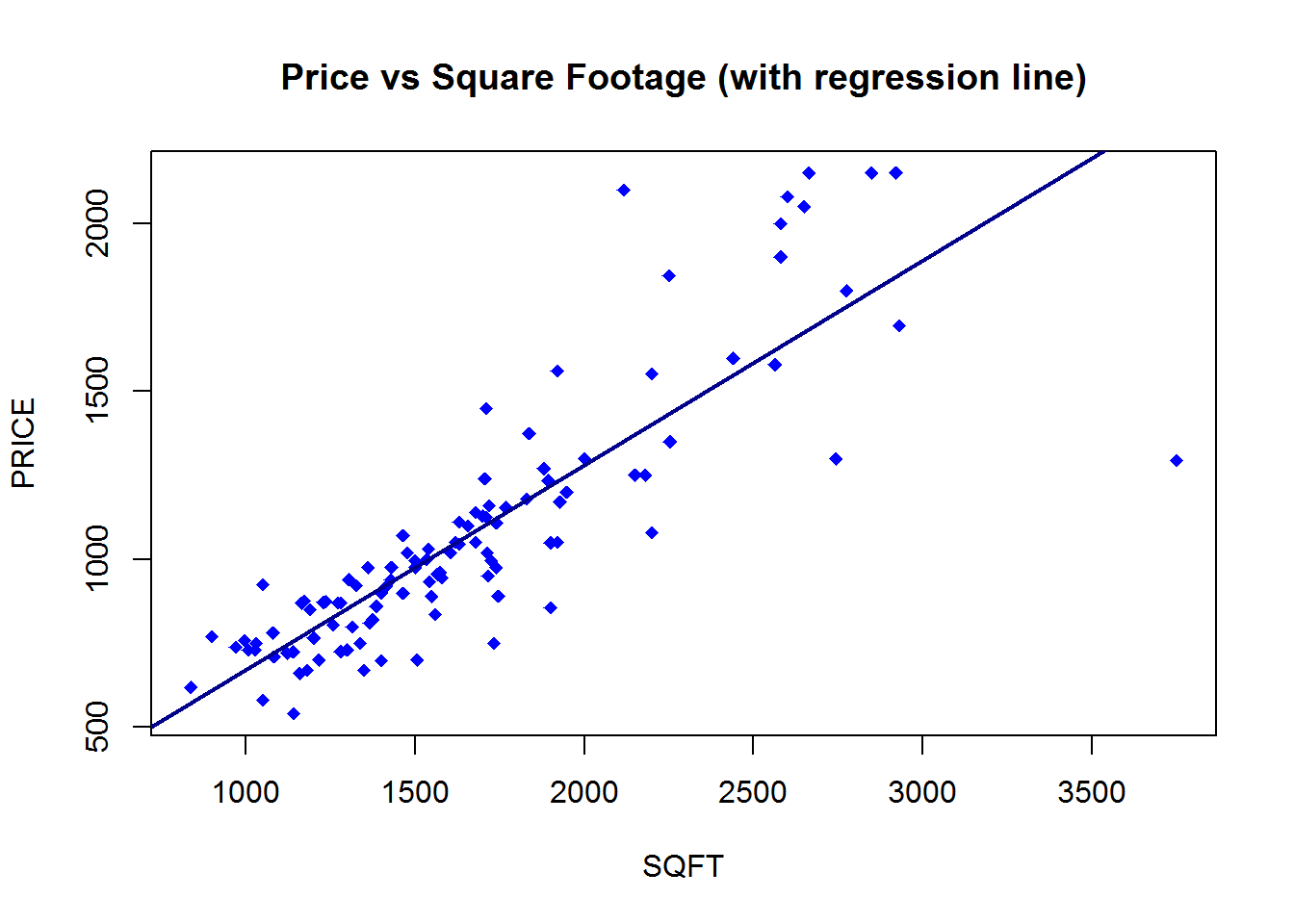Example of a real-world relationship (Source)

Our data similarly has a trend (which we call the true function) and random noise to make it more realistic. After creating the data, we split it into random training and testing sets. The model will attempt to learn the relationship on the training data and be evaluated on the test data. In this case, 70% of the data is used for training and 30% for testing. The following graph shows the data we will explore.

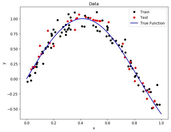Data and True Generating Funtion

We can see that our data are distributed with some variation around the true function (a partial sine wave) because of the random noise we added (see code for details). During training, we want our model to learn the true function without being “distracted” by the noise.

Model Building

Choosing a model can seem intimidating, but a good rule is to start simple and then build your way up. The simplest model is a linear regression, where the outputs are a linearly weighted combination of the inputs. In our model, we will use an extension of linear regression called polynomial regression to learn the relationship between x and y. Polynomial regression, where the inputs are raised to different powers, is still considered a form of “linear” regression even though the graph does not form a straight line (this confused me at first as well!)The general equation for a polynomial is below.

Here y represents the label and x is the feature. The beta terms are the model parameters which will be learned during training, and the epsilon is the error present in any model. Once the model has learned the beta values, we can plug in any value for x and get a corresponding prediction for y. A polynomial is defined by its order, which is the highest power of x in the equation. A straight line is a polynomial of degree 1 while a parabola has 2 degrees.

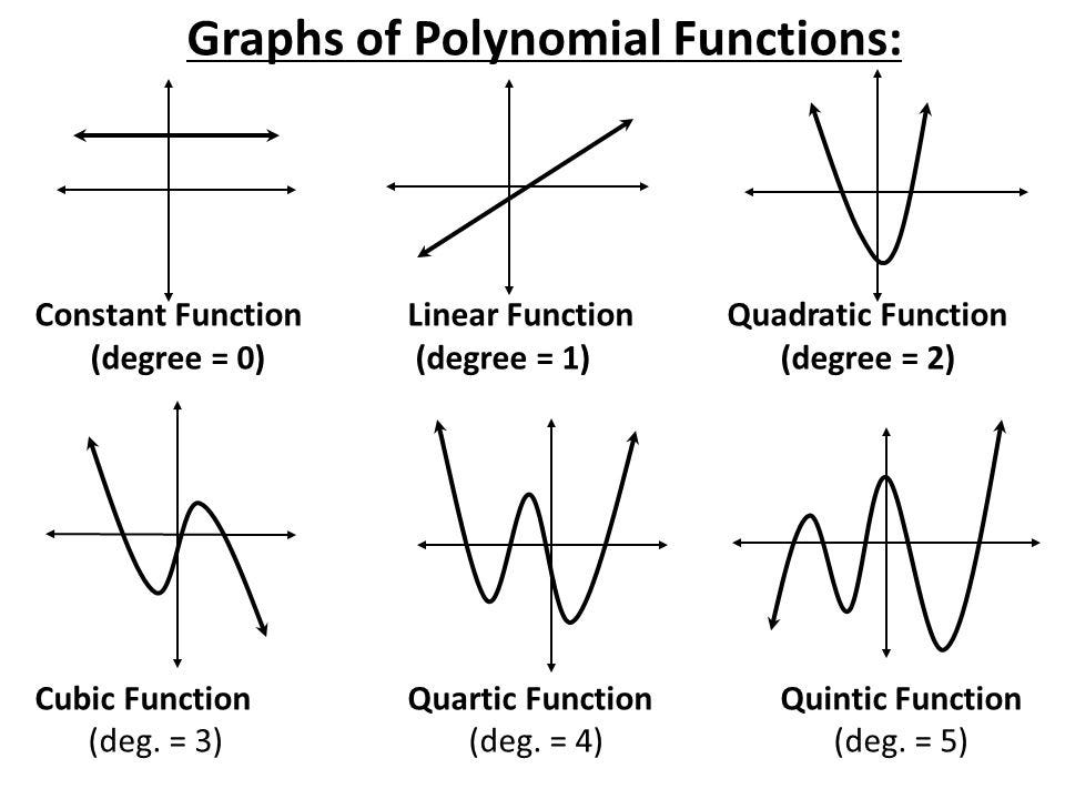Polynomials of Varying Degree (Source)

Overfitting vs. Underfitting

The problem of Overfitting vs Underfitting finally appears when we talk about the polynomial degree. The degree represents how much flexibility is in the model, with a higher power allowing the model freedom to hit as many data points as possible. An underfit model will be less flexible and cannot account for the data. The best way to understand the issue is to take a look at models demonstrating both situations.

First up is an underfit model with a 1 degree polynomial fit. In the image on the left, model function in orange is shown on top of the true function and the training observations. On the right, the model predictions for the testing data are shown compared to the true function and testing data points.

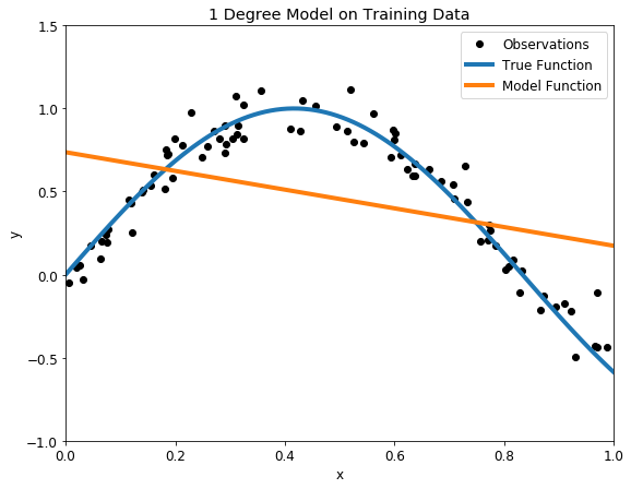
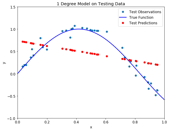Underfit 1 degree polynomial model on training (left) and testing (right) datasets

Our model passes straight through the training set with no regard for the data! This is because an underfit model has low variance and high bias. Variance refers to how much the model is dependent on the training data. For the case of a 1 degree polynomial, the model depends very little on the training data because it barely pays any attention to the points! Instead, the model has high bias, which means it makes a strong assumption about the data. For this example, the assumption is that the data is linear, which is evidently quite wrong. When the model makes test predictions, the bias leads it to make inaccurate estimates. The model failed to learn the relationship between x and y because of this bias, a clear example of underfitting.

We saw a low degree leads to underfitting. A natural conclusion would be to learn the training data, we should just increase the degree of the model to capture every change in the data. This however is not the best decision!

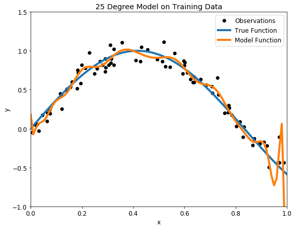
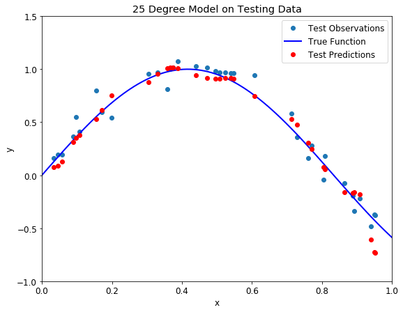Overfit 25 degree polynomial model on training (left) and testing (right) datasets

With such a high degree of flexibility, the model does its best to account for every single training point. This might seem like a good idea — don’t we want to learn from the data? Further, the model has a great score on the training data because it gets close to all the points. While this would be acceptable if the training observations perfectly represented the true function, because there is noise in the data, our model ends up fitting the noise. This is a model with a high variance, because it will change significantly depending on the training data. The predictions on the test set are better than the one degree model, but the twenty five degree model still does not learn the relationship because it essentially memorizes the training data and the noise.

Our problem is that we want a model that does not “memorize” the training data, but learns the actual relationship! How can we find a balanced model with the right polynomial degree? If we choose the model with the best score on the training set, we will just select the overfitting model but this cannot generalize well to testing data. Fortunately, there is a well-established data science technique for developing the optimal model: validation.

Validation

We need to create a model with the best settings (the degree), but we don’t want to have to keep going through training and testing. There are no consequences in our example from poor test performance, but in a real application where we might be performing a critical task such as diagnosing cancer, there would be serious downsides to deploying a faulty model. We need some sort of pre-test to use for model optimization and evaluate. This pre-test is known as a validation set.

A basic approach would be to use a validation set in addition to the training and testing set. This presents a few problems though: we could just end up overfitting to the validation set and we would have less training data. A smarter implementation of the validation concept is k-fold cross-validation.

The idea is straightforward: rather than using a separate validation set, we split the training set into a number of subsets, called folds. Let’s use five folds as an example. We perform a series of train and evaluate cycles where each time we train on 4 of the folds and test on the 5th, called the hold-out set. We repeat this cycle 5 times, each time using a different fold for evaluation. At the end, we average the scores for each of the folds to determine the overall performance of a given model. This allows us to optimize the model before deployment without having to use additional data.

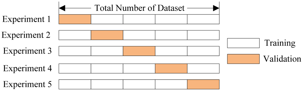Five-Fold Cross-Validation (Source)

For our problem, we can use cross-validation to select the best model by creating models with a range of different degrees, and evaluate each one using 5-fold cross-validation. The model with the lowest cross-validation score will perform best on the testing data and will achieve a balance between underfitting and overfitting. I choose to use models with degrees from 1 to 40 to cover a wide range. To compare models, we compute the mean-squared error, the average distance between the prediction and the real value squared. The following table shows the cross validation results ordered by lowest error and the graph shows all the results with error on the y-axis.

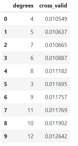
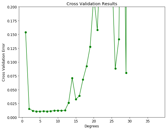Cross Validation Results

The cross-validation error with the underfit and overfit models is off the chart! A model with 4 degrees appears to be optimal. To test out the results, we can make a 4-degree model and view the training and testing predictions.

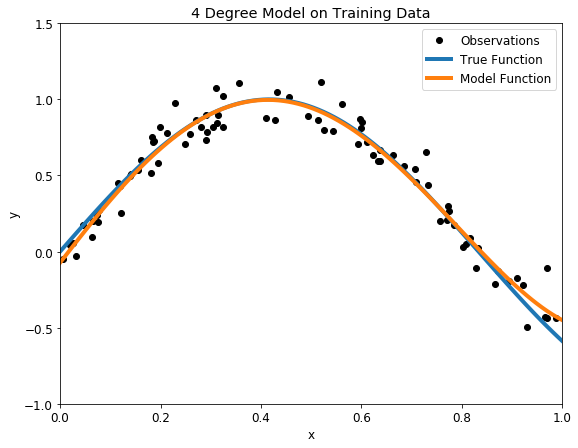
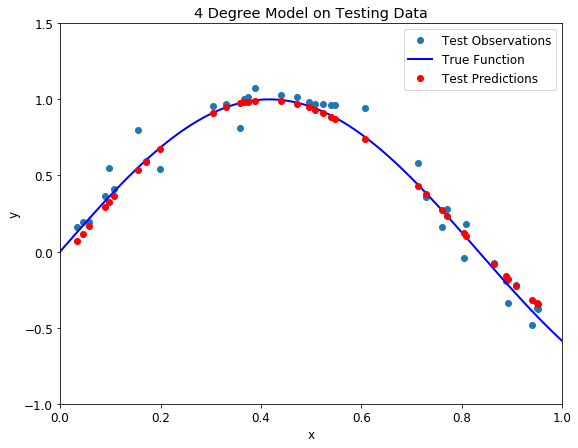Balanced Four degree polynomial model on training (left) and testing (right) datasets

There is nothing more beautiful than a model that fits the data! Moreover, we know that our model not only closely follows the training data, it has actually learned the relationship between x and y.

To verify we have the optimal model, we can also plot what are known as training and testing curves. These show the model setting we tuned on the x-axis and both the training and testing error on the y-axis. A model that is underfit will have high training and high testing error while an overfit model will have extremely low training error but a high testing error.

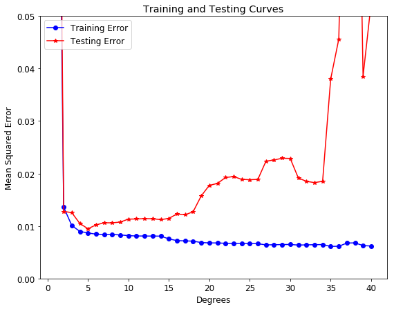Training and Testing Curves

This graph nicely summarizes the problem of overfitting and underfitting. As the flexibility in the model increases (by increasing the polynomial degree) the training error continually decreases due to increased flexibility. However, the error on the testing set only decreases as we add flexibility up to a certain point. In this case, that occurs at 5 degrees As the flexibility increases beyond this point, the training error increases because the model has memorized the training data and the noise. Cross-validation yielded the second best model on this testing data, but in the long run we expect our cross-validation model to perform best. The exact metrics depend on the testing set, but on average, the best model from cross-validation will outperform all other models.

Conclusions

Overfitting and underfitting is a fundamental problem that trips up even experienced data analysts. In my lab, I have seen many grad students fit a model with extremely low error to their data and then eagerly write a paper with the results. Their model looks great, but the problem is they never even used a testing set let alone a validation set! The model is nothing more than an overfit representation of the training data, a lesson the student soon learns when someone else tries to apply their model to new data.

Fortunately, this is a mistake that we can easily avoid now that we have seen the importance of model evaluation and optimization using cross-validation. Once we understand the basic problems in data science and how to address them, we can feel confident in building up more complex models and helping others avoid mistakes. This post covered a lot of topics, but hopefully you now have an idea of the basics of modeling, overfitting vs underfitting, bias vs variance, and model optimization with cross-validation. Data science is all about being willing to learn and continually adding more tools to your skillset. The field is exciting both for its potential beneficial impacts and for the opportunity to constantly learn new techniques.

I welcome feedback and constructive criticism. I can be reached on Twitter at @koehrsen_will. I would like to thank the contributors to Scikit-Learn for their excellent example on this subject.