(Source)

How to use a pre-trained convolutional neural network for object recognition with PyTorch

Although Keras is a great library with a simple API for building neural networks, the recent excitement about PyTorch finally got me interested in exploring this library. While I’m one to blindly follow the hype, the adoption by researchers and inclusion in the fast.ai library convinced me there must be something behind this new entry in deep learning.

Since the best way to learn a new technology is by using it to solve a problem, my efforts to learn PyTorch started out with a simple project: use a pre-trained convolutional neural network for an object recognition task. In this article, we’ll see how to use PyTorch to accomplish this goal, along the way, learning a little about the library and about the important concept of transfer learning.

While PyTorch might not be for everyone, at this point it’s impossible to say which deep learning library will come out on top, and being able to quickly learn and use different tools is crucial to succeed as a data scientist.

The complete code for this project is available as a Jupyter Notebook on GitHub. This project was born out of my participation in the Udacity PyTorch scholarship challenge.

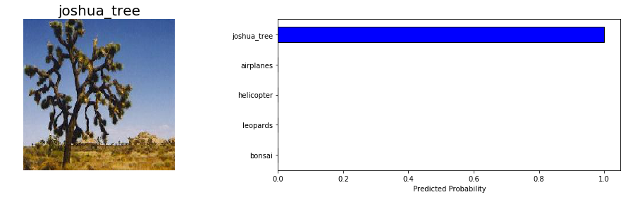Prediction from trained network

Approach to Transfer Learning

Our task will be to train a convolutional neural network (CNN) that can identify objects in images. We’ll be using the Caltech 101 dataset which has images in 101 categories. Most categories only have 50 images which typically isn’t enough for a neural network to learn to high accuracy. Therefore, instead of building and training a CNN from scratch, we’ll use a pre-built and pre-trained model applying transfer learning.

The basic premise of transfer learning is simple: take a model trained on a large dataset and transfer its knowledge to a smaller dataset. For object recognition with a CNN, we freeze the early convolutional layers of the network and only train the last few layers which make a prediction. The idea is the convolutional layers extract general, low-level features that are applicable across images — such as edges, patterns, gradients — and the later layers identify specific features within an image such as eyes or wheels.

Thus, we can use a network trained on unrelated categories in a massive dataset (usually Imagenet) and apply it to our own problem because there are universal, low-level features shared between images. The images in the Caltech 101 dataset are very similar to those in the Imagenet dataset and the knowledge a model learns on Imagenet should easily transfer to this task.

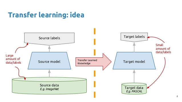Idea behind Transfer Learning (source).

Following is the general outline for transfer learning for object recognition:

1. Load in a pre-trained CNN model trained on a large dataset
2. Freeze parameters (weights) in model’s lower convolutional layers
3. Add custom classifier with several layers of trainable parameters to model
4. Train classifier layers on training data available for task
5. Fine-tune hyperparameters and unfreeze more layers as needed

This approach has proven successful for a wide range of domains. It’s a great tool to have in your arsenal and generally the first approach that should be tried when confronted with a new image recognition problem.

Data Set Up

With all data science problems, formatting the data correctly will determine the success or failure of the project. Fortunately, the Caltech 101 dataset images are clean and stored in the correct format. If we correctly set up the data directories, PyTorch makes it simple to associate the correct labels with each class. I separated the data into training, validation, and testing sets with a 50%, 25%, 25% split and then structured the directories as follows:

/datadir
    /train
        /class1
        /class2
        .
        .
    /valid
        /class1
        /class2
        .
        .
    /test
        /class1
        /class2
        .
        .

The number of training images by classes is below (I use the terms classes and categories interchangeably):

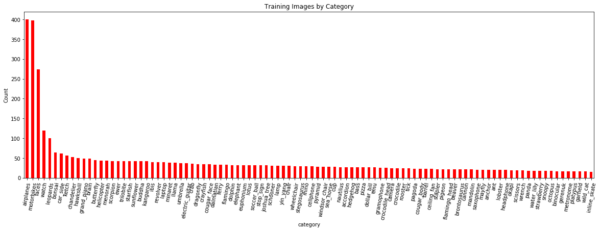Number of training images by category.

We expect the model to do better on classes with more examples because it can better learn to map features to labels. To deal with the limited number of training examples we’ll use data augmentation during training (more later).

As another bit of data exploration, we can also look at the size distribution.

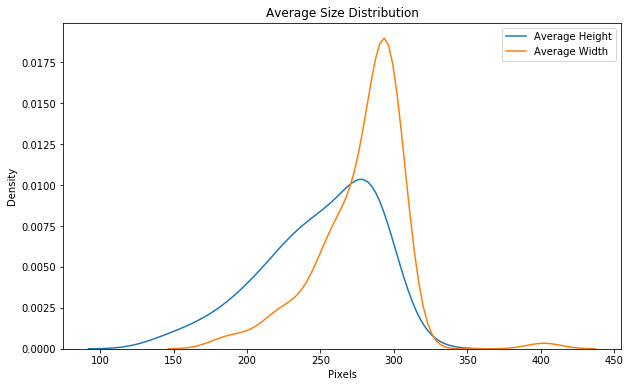Distribution of average image sizes (in pixels) by category.

Imagenet models need an input size of 224 x 224 so one of the preprocessing steps will be to resize the images. Preprocessing is also where we will implement data augmentation for our training data.

Data Augmentation

The idea of data augmentation is to artificially increase the number of training images our model sees by applying random transformations to the images. For example, we can randomly rotate or crop the images or flip them horizontally. We want our model to distinguish the objects regardless of orientation and data augmentation can also make a model invariant to transformations of the input data.

An elephant is still an elephant no matter which way it’s facing!

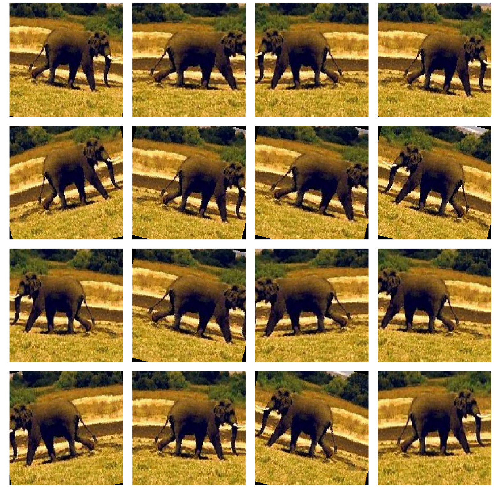Image transformations of training data.

Augmentation is generally only done during training (although test time augmentation is possible in the [fast.ai](https://blog.floydhub.com/ten-techniques-from-fast-ai/) library). Each epoch — one iteration through all the training images — a different random transformation is applied to each training image. This means that if we iterate through the data 20 times, our model will see 20 slightly different versions of each image. The overall result should be a model that learns the objects themselves and not how they are presented or artifacts in the image.

Image Preprocessing

This is the most important step of working with image data. During image preprocessing, we simultaneously prepare the images for our network and apply data augmentation to the training set. Each model will have different input requirements, but if we read through what Imagenet requires, we figure out that our images need to be 224x224 and normalized to a range.

To process an image in PyTorch, we use transforms , simple operations applied to arrays. The validation (and testing) transforms are as follows:

• Resize
• Center crop to 224 x 224
• Convert to a tensor
• Normalize with mean and standard deviation

The end result of passing through these transforms are tensors that can go into our network. The training transformations are similar but with the addition of random augmentations.

First up, we define the training and validation transformations:

Then, we create datasets and DataLoaders . By using datasets.ImageFolder to make a dataset, PyTorch will automatically associate images with the correct labels provided our directory is set up as above. The datasets are then passed to a DataLoader , an iterator that yield batches of images and labels.

We can see the iterative behavior of the DataLoader using the following:

# Iterate through the dataloader once
trainiter = iter(dataloaders['train'])
features, labels = next(trainiter)
features.shape, labels.shape

(torch.Size([128, 3, 224, 224]), torch.Size([128]))

The shape of a batch is (batch_size, color_channels, height, width). During training, validation, and eventually testing, we’ll iterate through the DataLoaders, with one pass through the complete dataset comprising one epoch. Every epoch, the training DataLoader will apply a slightly different random transformation to the images for training data augmentation.

Pre-Trained Models for Image Recognition

With our data in shape, we next turn our attention to the model. For this, we’ll use a pre-trained convolutional neural network. PyTorch has a number of models that have already been trained on millions of images from 1000 classes in Imagenet. The complete list of models can be seen here. The performance of these models on Imagenet is shown below:

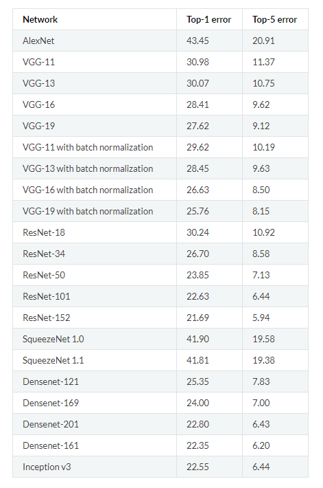Pretrained models in PyTorch and performance on Imagenet (Source).

For this implementation, we’ll be using the VGG-16. Although it didn’t record the lowest error, I found it worked well for the task and was quicker to train than other models. The process to use a pre-trained model is well-established:

1. Load in pre-trained weights from a network trained on a large dataset
2. Freeze all the weights in the lower (convolutional) layers: the layers to freeze are adjusted depending on similarity of new task to original dataset
3. Replace the upper layers of the network with a custom classifier: the number of outputs must be set equal to the number of classes
4. Train only the custom classifier layers for the task thereby optimizing the model for smaller dataset

Loading in a pre-trained model in PyTorch is simple:

from torchvision import models
model = model.vgg16(pretrained=True)

This model has over 130 million parameters, but we’ll train only the very last few fully-connected layers. Initially, we freeze all of the model’s weights:

# Freeze model weights
for param in model.parameters():
    param.requires_grad = False

Then, we add on our own custom classifier with the following layers:

• Fully connected with ReLU activation, shape = (n_inputs, 256)
• Dropout with 40% chance of dropping
• Fully connected with log softmax output, shape = (256, n_classes)

import torch.nn as nn
# Add on classifier
model.classifier[6] = nn.Sequential(
                      nn.Linear(n_inputs, 256),
                      nn.ReLU(),
                      nn.Dropout(0.4),
                      nn.Linear(256, n_classes),
                      nn.LogSoftmax(dim=1))

When the extra layers are added to the model, they are set to trainable by default ( require_grad=True ). For the VGG-16, we’re only changing the very last original fully-connected layer. All of the weights in the convolutional layers and the the first 5 fully-connected layers are not trainable.

# Only training classifier[6]
model.classifier

Sequential(
  (0): Linear(in_features=25088, out_features=4096, bias=True)
  (1): ReLU(inplace)
  (2): Dropout(p=0.5)
  (3): Linear(in_features=4096, out_features=4096, bias=True)
  (4): ReLU(inplace)
  (5): Dropout(p=0.5)
  (6): Sequential(
    (0): Linear(in_features=4096, out_features=256, bias=True)
    (1): ReLU()
    (2): Dropout(p=0.4)
    (3): Linear(in_features=256, out_features=100, bias=True)
    (4): LogSoftmax()
  )
)

The final outputs from the network are log probabilities for each of the 100 classes in our dataset. The model has a total of 135 million parameters, of which just over 1 million will be trained.

# Find total parameters and trainable parameters
total_params = sum(p.numel() for p in model.parameters())
print(f'{total_params:,} total parameters.')
total_trainable_params = sum(
    p.numel() for p in model.parameters() if p.requires_grad)
print(f'{total_trainable_params:,} training parameters.')

135,335,076 total parameters.
1,074,532 training parameters.

Moving Model to GPU(s)

One of the best aspects of PyTorch is the ease of moving different parts of a model to one or more gpus so you can make full use of your hardware. Since I’m using 2 gpus for training, I first move the model to cuda and then create a DataParallel model distributed over the gpus:

# Move to gpu
model = model.to('cuda')
# Distribute across 2 gpus
model = nn.DataParallel(model)

(This notebook should be run on a gpu to complete in a reasonable amount of time. The speedup over a cpu can easily by 10x or more.)

Training Loss and Optimizer

The training loss (the error or difference between predictions and true values) is the negative log likelihood (NLL). (The NLL loss in PyTorch expects log probabilities, so we pass in the raw output from the model’s final layer.) PyTorch uses automatic differentiation which means that tensors keep track of not only their value, but also every operation (multiply, addition, activation, etc.) which contributes to the value. This means we can compute the gradient for any tensor in the network with respect to any prior tensor.

What this means in practice is that the loss tracks not only the error, but also the contribution to the error by each weight and bias in the model. After we calculate the loss, we can then find the gradients of the loss with respect to each model parameter, a process known as backpropagation. Once we have the gradients, we use them to update the parameters with the optimizer. (If this doesn’t sink in at first, don’t worry, it takes a little while to grasp! This powerpoint helps to clarify some points.)

The optimizer is Adam, an efficient variant of gradient descent that generally does not require hand-tuning the learning rate. During training, the optimizer uses the gradients of the loss to try and reduce the error (“optimize”) of the model output by adjusting the parameters. Only the parameters we added in the custom classifier will be optimized.

The loss and optimizer are initialized as follows:

from torch import optim

# Loss and optimizer
criteration = nn.NLLLoss()
optimizer = optim.Adam(model.parameters())

With the pre-trained model, the custom classifier, the loss, the optimizer, and most importantly, the data, we’re ready for training.

Training

Model training in PyTorch is a little more hands-on than in Keras because we have to do the backpropagation and parameter update step ourselves. The main loop iterates over a number of epochs and on each epoch we iterate through the train DataLoader . The DataLoader yields one batch of data and targets which we pass through the model. After each training batch, we calculate the loss, backpropagate the gradients of the loss with respect to the model parameters, and then update the parameters with the optimizer.

I’d encourage you to look at the notebook for the complete training details, but the basic pseudo-code is as follows:

We can continue to iterate through the data until we reach a given number of epochs. However, one problem with this approach is that our model will eventually start overfitting to the training data. To prevent this, we use our validation data and early stopping.

Early Stopping

Early stopping means halting training when the validation loss has not decreased for a number of epochs. As we continue training, the training loss will only decrease, but the validation loss will eventually reach a minimum and plateau or start to increase. We ideally want to stop training when the validation loss is at a minimum in the hope that this model will generalize best to the testing data. When using early stopping, every epoch in which the validation loss decreases, we save the parameters so we can later retrieve those with the best validation performance.

We implement early stopping by iterating through the validation DataLoader at the end of each training epoch. We calculate the validation loss and compare this to the lowest validation loss. If the loss is the lowest so far, we save the model. If the loss has not improved for a certain number of epochs, we halt training and return the best model which has been saved to disk.

Again, the complete code is in the notebook, but pseudo-code is:

To see the benefits of early stopping, we can look at the training curves showing the training and validation losses and accuracy:

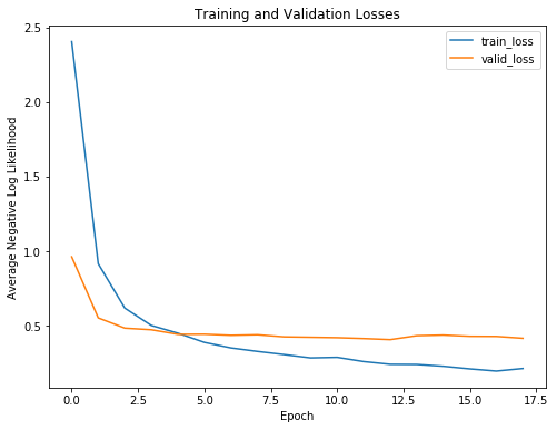
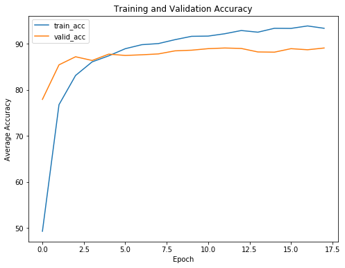Negative log likelihood and accuracy training curves

As expected, the training loss only continues to decrease with further training. The validation loss, on the other hand, reaches a minimum and plateaus. At a certain epoch, there is no return (or even a negative return) to further training. Our model will only start to memorize the training data and will not be able to generalize to testing data.

Without early stopping, our model will train for longer than necessary and will overfit to the training data.

Another point we can see from the training curves is that our model is not overfitting greatly. There is some overfitting as is always be the case, but the dropout after the first trainable fully connected layer prevents the training and validation losses from diverging too much.

Making Predictions: Inference

In the notebook I take care of some boring — but necessary — details of saving and loading PyTorch models, but here we’ll move right to the best part: making predictions on new images. We know our model does well on training and even validation data, but the ultimate test is how it performs on a hold-out testing set it has not seen before. We saved 25% of the data for the purpose of determining if our model can generalize to new data.

Predicting with a trained model is pretty simple. We use the same syntax as for training and validation:

for data, targets in testloader:
    log_ps = model(data)
    # Convert to probabilities
    ps = torch.exp(log_ps)

ps.shape()

(128, 100)

The shape of our probabilities are ( batch_size , n_classes ) because we have a probability for every class. We can find the accuracy by finding the highest probability for each example and compare these to the labels:

# Find predictions and correct
pred = torch.max(ps, dim=1)
equals = pred == targets

# Calculate accuracy
accuracy = torch.mean(equals)

When diagnosing a network used for object recognition, it can be helpful to look at both overall performance on the test set and individual predictions.

Model Results

Here are two predictions the model nails:

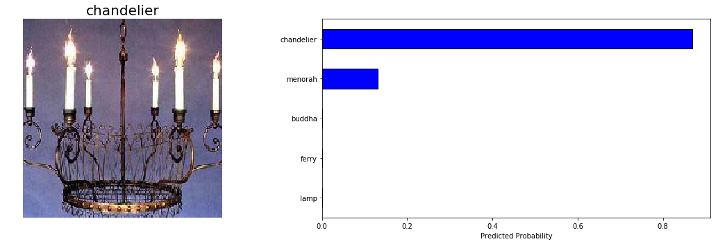
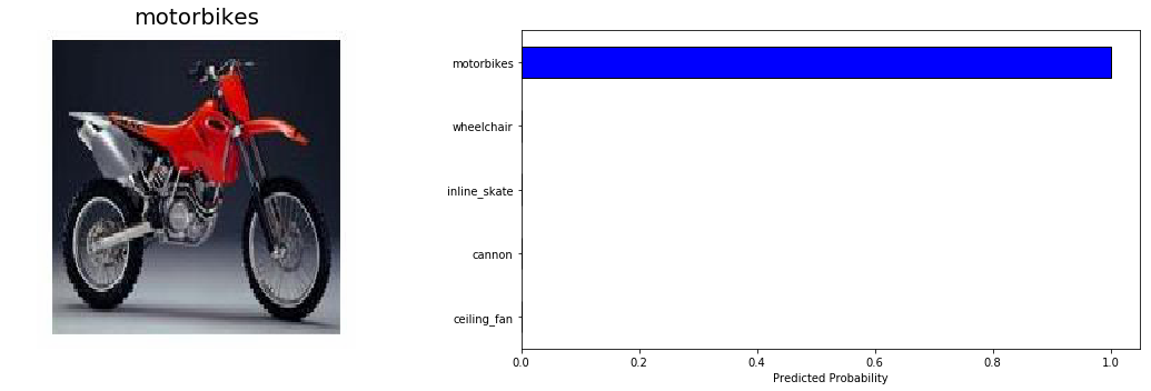Model Example Predictions

These are pretty easy, so I’m glad the model has no trouble!

We don’t just want to focus on the correct predictions and we’ll take a look at some wrong outputs shortly. For now let’s evaluate the performance on the entire test set. For this, we want to iterate over the test DataLoader and calculate the loss and accuracy for every example.

Convolutional neural networks for object recognition are generally measured in terms of topk accuracy. This refers to the whether or not the real class was in the k most likely predicted classes. For example, top 5 accuracy is the % the right class was in the 5 highest probability predictions. You can get the topk most likely probabilities and classes from a PyTorch tensor as follows:

top_5_ps, top_5_classes = ps.topk(5, dim=1)
top_5_ps.shape

(128, 5)

Evaluating the model on the entire testing set, we calculate the metrics:

Final test top 1 weighted accuracy = 88.65%
Final test top 5 weighted accuracy = 98.00%
Final test cross entropy per image = 0.3772.

These compare favorably to the near 90% top 1 accuracy on the validation data. Overall, we conclude our pre-trained model was able to successfully transfer its knowledge from Imagenet to our smaller dataset.

Model Investigation

Although the model does well, there’s likely steps to take which can make it even better. Often, the best way to figure out how to improve a model is to investigate its errors (note: this is also an effective self-improvement method.)

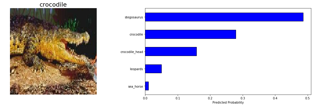
Our model isn’t great at identifying crocodiles, so let’s look at some test predictions from this category:

![] (https://cdn-images-1.medium.com/max/2000/1kEmyc_lZ0TWYOgvgLlUsqw.png) 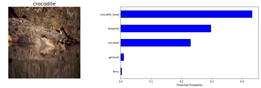*Model Example Predictions

Given the subtle distinction between crocodile and crocodile_head , and the difficulty of the second image, I’d say our model is not entirely unreasonable in these predictions. The ultimate goal in image recognition is to exceed human capabilities, and our model is nearly there!

Finally, we’d expect the model to perform better on categories with more images, so we can look at a graph of accuracy in a given category versus the number of training images in that category:

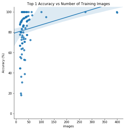
There does appear to be a positive correlation between the number of training images and the top 1 test accuracy. This indicates that _more training data augmentation could be helpfu_l, or, even that we should use test time augmentation. We could also try a different pre-trained model, or build another custom classifier. At the moment, deep learning is still an empirical field meaning experimentation is often required!

Conclusions

While there are easier deep learning libraries to use, the benefits of PyTorch are speed, control over every aspect of model architecture / training, efficient implementation of backpropagation with tensor auto differentiation, and ease of debugging code due to the dynamic nature of PyTorch graphs. For production code or your own projects, I’m not sure there is yet a compelling argument for using PyTorch instead of a library with a gentler learning curve such as Keras, but it’s helpful to know how to use different options.

Through this project, we were able to see the basics of using PyTorch as well as the concept of transfer learning, an effective method for object recognition. Instead of training a model from scratch, we can use existing architectures that have been trained on a large dataset and then tune them for our task. This reduces the time to train and often results in better overall performance. The outcome of this project is some knowledge of transfer learning and PyTorch that we can build on to build more complex applications.

We truly live in an incredible age for deep learning, where anyone can build deep learning models with easily available resources! Now get out there and take advantage of these resources by building your own project.

As always, I welcome feedback and constructive criticism. I can be reached on Twitter @koehrsen_will or through my personal website willk.online.