Model Selection, Hyperparameter Tuning, and Evaluation

Assembling all the machine learning pieces needed to solve a problem can be a daunting task. In this series of articles, we are walking through implementing a machine learning workflow using a real-world dataset to see how the individual techniques come together.

In the first post, we cleaned and structured the data, performed an exploratory data analysis, developed a set of features to use in our model, and established a baseline against which we can measure performance. In this article, we will look at how to implement and compare several machine learning models in Python, perform hyperparameter tuning to optimize the best model, and evaluate the final model on the test set.

The full code for this project is on GitHub and the second notebook corresponding to this article is here. Feel free to use, share, and modify the code in any way you want!

Model Evaluation and Selection

As a reminder, we are working on a supervised regression task: using New York City building energy data, we want to develop a model that can predict the Energy Star Score of a building. Our focus is on both accuracy of the predictions and interpretability of the model.

There are a ton of machine learning models to choose from and deciding where to start can be intimidating. While there are some charts that try to show you which algorithm to use, I prefer to just try out several and see which one works best! Machine learning is still a field driven primarily by empirical (experimental) rather than theoretical results, and it’s almost impossible to know ahead of time which model will do the best.

Generally, it’s a good idea to start out with simple, interpretable models such as linear regression, and if the performance is not adequate, move on to more complex, but usually more accurate methods. The following chart shows a (highly unscientific) version of the accuracy vs interpretability trade-off:

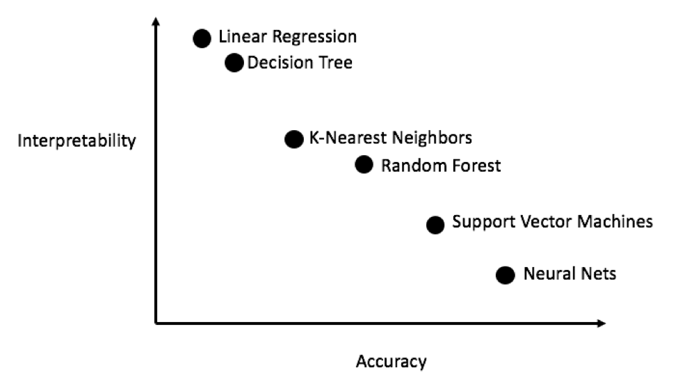Interpretability vs. Accuracy (Source)

We will evaluate five different models covering the complexity spectrum:

• Linear Regression
• K-Nearest Neighbors Regression
• Random Forest Regression
• Gradient Boosted Regression
• Support Vector Machine Regression

In this post we will focus on implementing these methods rather than the theory behind them. For anyone interesting in learning the background, I highly recommend An Introduction to Statistical Learning (available free online) or Hands-On Machine Learning with Scikit-Learn and TensorFlow. Both of these textbooks do a great job of explaining the theory and showing how to effectively use the methods in R and Python respectively.

Imputing Missing Values

While we dropped the columns with more than 50% missing values when we cleaned the data, there are still quite a few missing observations. Machine learning models cannot deal with any absent values, so we have to fill them in, a process known as imputation.

First, we’ll read in all the data and remind ourselves what it looks like:

import pandas as pd
import numpy as np

# Read in data into dataframes
train_features = pd.read_csv('data/training_features.csv')
test_features = pd.read_csv('data/testing_features.csv')
train_labels = pd.read_csv('data/training_labels.csv')
test_labels = pd.read_csv('data/testing_labels.csv')

**Training Feature Size:  (6622, 64)
Testing Feature Size:   (2839, 64)
Training Labels Size:   (6622, 1)
Testing Labels Size:    (2839, 1)**

Every value that is NaN represents a missing observation. While there are a number of ways to fill in missing data, we will use a relatively simple method, median imputation. This replaces all the missing values in a column with the median value of the column.

In the following code, we create a Scikit-Learn Imputer object with the strategy set to median. We then train this object on the training data (using imputer.fit) and use it to fill in the missing values in both the training and testing data (using imputer.transform). This means missing values in the test data are filled in with the corresponding median value from the training data.

(We have to do imputation this way rather than training on all the data to avoid the problem of test data leakage, where information from the testing dataset spills over into the training data.)

# Create an imputer object with a median filling strategy
imputer = Imputer(strategy='median')

# Train on the training features
imputer.fit(train_features)

# Transform both training data and testing data
X = imputer.transform(train_features)
X_test = imputer.transform(test_features)

**Missing values in training features:  0
Missing values in testing features:   0**

All of the features now have real, finite values with no missing examples.

Feature Scaling

Scaling refers to the general process of changing the range of a feature. This is necessary because features are measured in different units, and therefore cover different ranges. Methods such as support vector machines and K-nearest neighbors that take into account distance measures between observations are significantly affected by the range of the features and scaling allows them to learn. While methods such as Linear Regression and Random Forest do not actually require feature scaling, it is still best practice to take this step when we are comparing multiple algorithms.

We will scale the features by putting each one in a range between 0 and 1. This is done by taking each value of a feature, subtracting the minimum value of the feature, and dividing by the maximum minus the minimum (the range). This specific version of scaling is often called normalization and the other main version is known as standardization.

While this process would be easy to implement by hand, we can do it using a MinMaxScaler object in Scikit-Learn. The code for this method is identical to that for imputation except with a scaler instead of imputer! Again, we make sure to train only using training data and then transform all the data.

# Create the scaler object with a range of 0-1
scaler = MinMaxScaler(feature_range=(0, 1))

# Fit on the training data
scaler.fit(X)

# Transform both the training and testing data
X = scaler.transform(X)
X_test = scaler.transform(X_test)

Every feature now has a minimum value of 0 and a maximum value of 1. Missing value imputation and feature scaling are two steps required in nearly any machine learning pipeline so it’s a good idea to understand how they work!

Implementing Machine Learning Models in Scikit-Learn

After all the work we spent cleaning and formatting the data, actually creating, training, and predicting with the models is relatively simple. We will use the Scikit-Learn library in Python, which has great documentation and a consistent model building syntax. Once you know how to make one model in Scikit-Learn, you can quickly implement a diverse range of algorithms.

We can illustrate one example of model creation, training (using .fit ) and testing (using .predict ) with the Gradient Boosting Regressor:

**Gradient Boosted Performance on the test set: MAE = 10.0132**

Model creation, training, and testing are each one line! To build the other models, we use the same syntax, with the only change the name of the algorithm. The results are presented below:

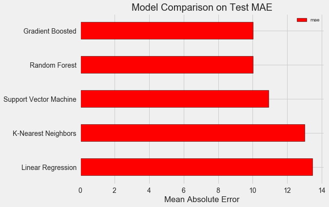To put these figures in perspective, the naive baseline calculated using the median value of the target was 24.5. Clearly, machine learning is applicable to our problem because of the significant improvement over the baseline!

The gradient boosted regressor (MAE = 10.013) slightly beats out the random forest (10.014 MAE). These results aren’t entirely fair because we are mostly using the default values for the hyperparameters. Especially in models such as the support vector machine, the performance is highly dependent on these settings. Nonetheless, from these results we will select the gradient boosted regressor for model optimization.

Hyperparameter Tuning for Model Optimization

In machine learning, after we have selected a model, we can optimize it for our problem by tuning the model hyperparameters.

First off, what are hyperparameters and how do they differ from parameters?

• Model hyperparameters are best thought of as settings for a machine learning algorithm that are set by the data scientist before training. Examples would be the number of trees in a random forest or the number of neighbors used in K-nearest neighbors algorithm.
• Model parameters are what the model learns during training, such as weights in a linear regression.

Controlling the hyperparameters affects the model performance by altering the balance between underfitting and overfitting in a model. Underfitting is when our model is not complex enough (it does not have enough degrees of freedom) to learn the mapping from features to target. An underfit model has high bias, which we can correct by making our model more complex.

Overfitting is when our model essentially memorizes the training data. An overfit model has high variance, which we can correct by limiting the complexity of the model through regularization. Both an underfit and an overfit model will not be able to generalize well to the testing data.

The problem with choosing the right hyperparameters is that the optimal set will be different for every machine learning problem! Therefore, the only way to find the best settings is to try out a number of them on each new dataset. Luckily, Scikit-Learn has a number of methods to allow us to efficiently evaluate hyperparameters. Moreover, projects such as TPOT by Epistasis Lab are trying to optimize the hyperparameter search using methods like genetic programming. In this project, we will stick to doing this with Scikit-Learn, but stayed tuned for more work on the auto-ML scene!

Random Search with Cross Validation

The particular hyperparameter tuning method we will implement is called random search with cross validation:

• Random Search refers to the technique we will use to select hyperparameters. We define a grid and then randomly sample different combinations, rather than grid search where we exhaustively try out every single combination. (Surprisingly, random search performs nearly as well as grid search with a drastic reduction in run time.)
• Cross Validation is the technique we use to evaluate a selected combination of hyperparameters. Rather than splitting the training set up into separate training and validation sets, which reduces the amount of training data we can use, we use K-Fold Cross Validation. This involves dividing the training data into K number of folds, and then going through an iterative process where we first train on K-1 of the folds and then evaluate performance on the Kth fold. We repeat this process K times and at the end of K-fold cross validation, we take the average error on each of the K iterations as the final performance measure.

The idea of K-Fold cross validation with K = 5 is shown below:

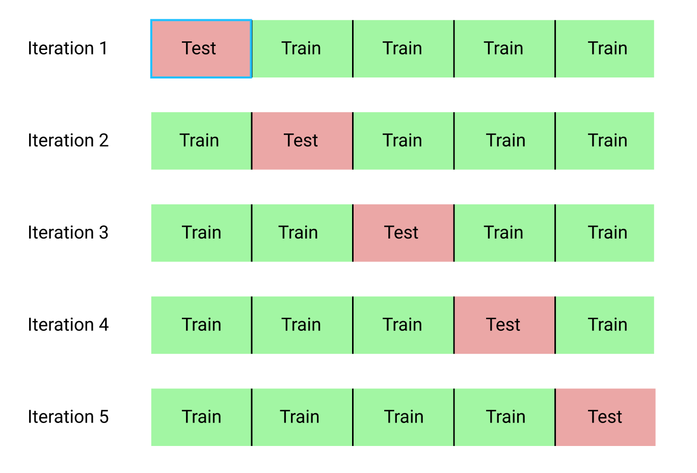K-Fold Cross Validation with K = 5 (Source)

The entire process of performing random search with cross validation is:

1. Set up a grid of hyperparameters to evaluate
2. Randomly sample a combination of hyperparameters
3. Create a model with the selected combination
4. Evaluate the model using K-fold cross validation
5. Decide which hyperparameters worked the best

Of course, we don’t do actually do this manually, but rather let Scikit-Learn’s RandomizedSearchCV handle all the work!

Slight Diversion: Gradient Boosted Methods

Since we will be using the Gradient Boosted Regression model, I should give at least a little background! This model is an ensemble method, meaning that it is built out of many weak learners, in this case individual decision trees. While a bagging algorithm such as random forest trains the weak learners in parallel and has them vote to make a prediction, a boosting method like Gradient Boosting, trains the learners in sequence, with each learner “concentrating” on the mistakes made by the previous ones.

Boosting methods have become popular in recent years and frequently win machine learning competitions. The Gradient Boosting Method is one particular implementation that uses Gradient Descent to minimize the cost function by sequentially training learners on the residuals of previous ones. The Scikit-Learn implementation of Gradient Boosting is generally regarded as less efficient than other libraries such as XGBoost , but it will work well enough for our small dataset and is quite accurate.

Back to Hyperparameter Tuning

There are many hyperparameters to tune in a Gradient Boosted Regressor and you can look at the Scikit-Learn documentation for the details. We will optimize the following hyperparameters:

• loss: the loss function to minimize
• n_estimators: the number of weak learners (decision trees) to use
• max_depth: the maximum depth of each decision tree
• min_samples_leaf: the minimum number of examples required at a leaf node of the decision tree
• min_samples_split: the minimum number of examples required to split a node of the decision tree
• max_features: the maximum number of features to use for splitting nodes

I’m not sure if there is anyone who truly understands how all of these interact, and the only way to find the best combination is to try them out!

In the following code, we build a hyperparameter grid, create a RandomizedSearchCV object, and perform hyperparameter search using 4-fold cross validation over 25 different combinations of hyperparameters:

After performing the search, we can inspect the RandomizedSearchCV object to find the best model:

# Find the best combination of settings
random_cv.best_estimator_

**GradientBoostingRegressor(loss='lad', max_depth=5,
                          max_features=None,
                          min_samples_leaf=6,
                          min_samples_split=6,
                          n_estimators=500)**

We can then use these results to perform grid search by choosing parameters for our grid that are close to these optimal values. However, further tuning is unlikely to significant improve our model. As a general rule, proper feature engineering will have a much larger impact on model performance than even the most extensive hyperparameter tuning. It’s the law of diminishing returns applied to machine learning: feature engineering gets you most of the way there, and hyperparameter tuning generally only provides a small benefit.

One experiment we can try is to change the number of estimators (decision trees) while holding the rest of the hyperparameters steady. This directly lets us observe the effect of this particular setting. See the notebook for the implementation, but here are the results:

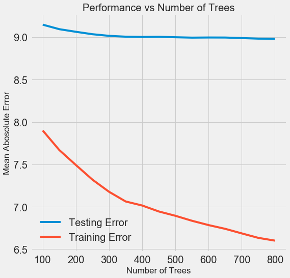As the number of trees used by the model increases, both the training and the testing error decrease. However, the training error decreases much more rapidly than the testing error and we can see that our model is overfitting: it performs very well on the training data, but is not able to achieve that same performance on the testing set.

We always expect at least some decrease in performance on the testing set (after all, the model can see the true answers for the training set), but a significant gap indicates overfitting. We can address overfitting by getting more training data, or decreasing the complexity of our model through the hyerparameters. In this case, we will leave the hyperparameters where they are, but I encourage anyone to try and reduce the overfitting.

For the final model, we will use 800 estimators because that resulted in the lowest error in cross validation. Now, time to test out this model!

Evaluating on the Test Set

As responsible machine learning engineers, we made sure to not let our model see the test set at any point of training. Therefore, we can use the test set performance as an indicator of how well our model would perform when deployed in the real world.

Making predictions on the test set and calculating the performance is relatively straightforward. Here, we compare the performance of the default Gradient Boosted Regressor to the tuned model:

# Make predictions on the test set using default and final model
default_pred = default_model.predict(X_test)
final_pred = final_model.predict(X_test)

**Default model performance on the test set: MAE = 10.0118.
Final model performance on the test set:   MAE = 9.0446.**

Hyperparameter tuning improved the accuracy of the model by about 10%. Depending on the use case, 10% could be a massive improvement, but it came at a significant time investment!

We can also time how long it takes to train the two models using the %timeit magic command in Jupyter Notebooks. First is the default model:

%%timeit -n 1 -r 5
default_model.fit(X, y)

**1.09 s ± 153 ms per loop (mean ± std. dev. of 5 runs, 1 loop each)**

1 second to train seems very reasonable. The final tuned model is not so fast:

%%timeit -n 1 -r 5
final_model.fit(X, y)

**12.1 s ± 1.33 s per loop (mean ± std. dev. of 5 runs, 1 loop each)**

This demonstrates a fundamental aspect of machine learning: it is always a game of trade-offs. We constantly have to balance accuracy vs interpretability, bias vs variance, accuracy vs run time, and so on. The right blend will ultimately depend on the problem. In our case, a 12 times increase in run-time is large in relative terms, but in absolute terms it’s not that significant.

Once we have the final predictions, we can investigate them to see if they exhibit any noticeable skew. On the left is a density plot of the predicted and actual values, and on the right is a histogram of the residuals:

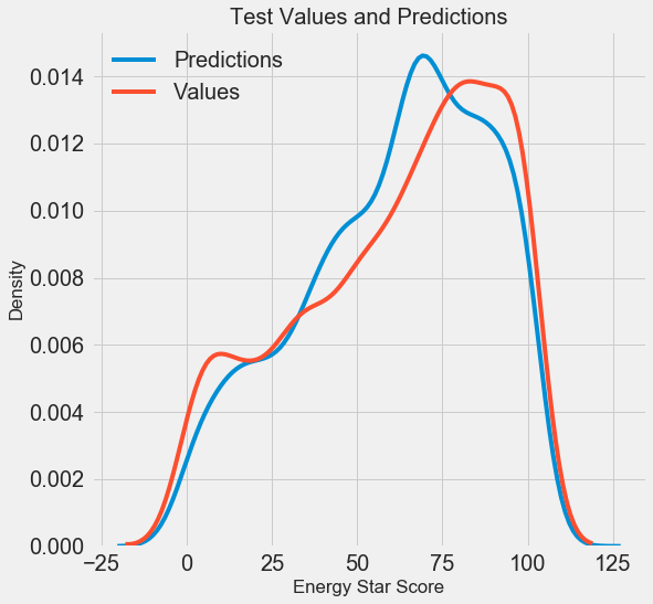
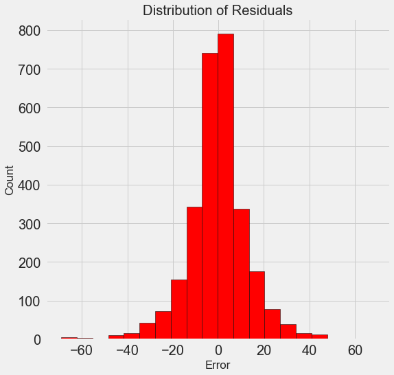Density Plot of Predicted and Actual Values (left) and Histogram of Residuals (right)

The model predictions seem to follow the distribution of the actual values although the peak in the density occurs closer to the median value (66) on the training set than to the true peak in density (which is near 100). The residuals are nearly normally distribution, although we see a few large negative values where the model predictions were far below the true values. We will take a deeper look at interpreting the results of the model in the next post.

Conclusions

In this article we covered several steps in the machine learning workflow:

• Imputation of missing values and scaling of features
• Evaluating and comparing several machine learning models
• Hyperparameter tuning using random grid search and cross validation
• Evaluating the best model on the test set

The results of this work showed us that machine learning is applicable to the task of predicting a building’s Energy Star Score using the available data. Using a gradient boosted regressor we were able to predict the scores on the test set to within 9.1 points of the true value. Moreover, we saw that hyperparameter tuning can increase the performance of a model at a significant cost in terms of time invested. This is one of many trade-offs we have to consider when developing a machine learning solution.

In the third post (available here), we will look at peering into the black box we have created and try to understand how our model makes predictions. We also will determine the greatest factors influencing the Energy Star Score. While we know that our model is accurate, we want to know why it makes the predictions it does and what this tells us about the problem!

As always, I welcome feedback and constructive criticism and can be reached on Twitter @koehrsen_will.