Interpreting a machine learning model and presenting results

Machine learning models are often criticized as black boxes: we put data in one side, and get out answers — often very accurate answers — with no explanations on the other. In the third part of this series showing a complete machine learning solution, we will peer into the model we developed to try and understand how it makes predictions and what it can teach us about the problem. We will wrap up by discussing perhaps the most important part of a machine learning project: documenting our work and presenting results.

Part one of the series covered data cleaning, exploratory data analysis, feature engineering, and feature selection. Part two covered imputing missing values, implementing and comparing machine learning models, hyperparameter tuning using random search with cross validation, and evaluating a model.

All the code for this project is on GitHub. The third Jupyter Notebook, corresponding to this post, is here. I encourage anyone to share, use, and build on this code!

As a reminder, we are working through a supervised regression machine learning problem. Using New York City building energy data, we have developed a model which can predict the Energy Star Score of a building. The final model we built is a Gradient Boosted Regressor which is able to predict the Energy Star Score on the test data to within 9.1 points (on a 1–100 scale).

Model Interpretation

The gradient boosted regressor sits somewhere in the middle on the scale of model interpretability: the entire model is complex, but it is made up of hundreds of decision trees, which by themselves are quite understandable. We will look at three ways to understand how our model makes predictions:

1. Feature importances
2. Visualizing a single decision tree
3. LIME: Local Interpretable Model-Agnostic Explainations

The first two methods are specific to ensembles of trees, while the third — as you might have guessed from the name — can be applied to any machine learning model. LIME is a relatively new package and represents an exciting step in the ongoing effort to explain machine learning predictions.

Feature Importances

Feature importances attempt to show the relevance of each feature to the task of predicting the target. The technical details of feature importances are complex (they measure the mean decrease impurity, or the reduction in error from including the feature), but we can use the relative values to compare which features are the most relevant. In Scikit-Learn, we can extract the feature importances from any ensemble of tree-based learners.

With model as our trained model, we can find the feature importances usingmodel.feature_importances_ . Then we can put them into a pandas DataFrame and display or plot the top ten most important:

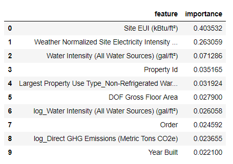
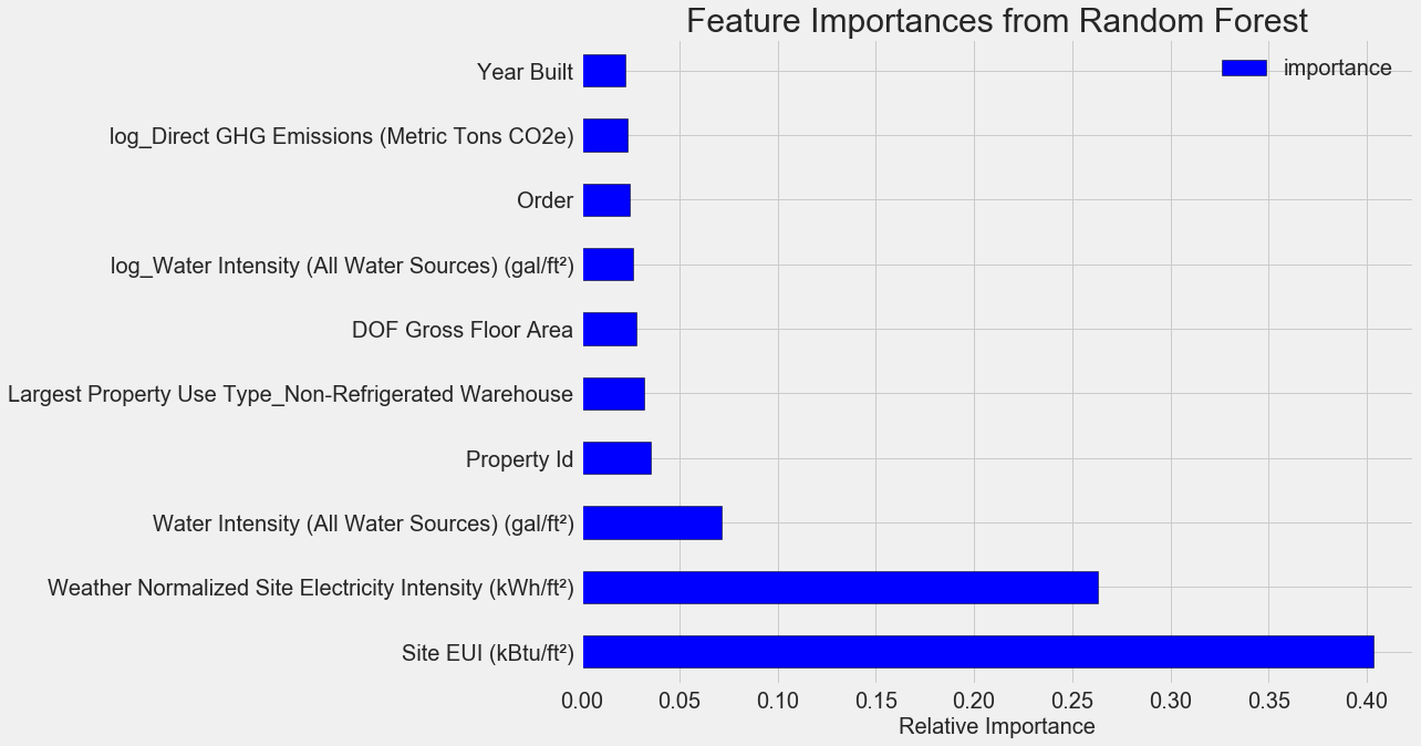The Site EUI(Energy Use Intensity) and the Weather Normalized Site Electricity Intensity are by far the most important features, accounting for over 66% of the total importance. After the top two features, the importance drops off significantly, which indicates we might not need to retain all 64 features in the data to achieve high performance. (In the Jupyter notebook, I take a look at using only the top 10 features and discover that the model is not quite as accurate.)

Based on these results, we can finally answer one of our initial questions: the most important indicators of a building’s Energy Star Score are the Site EUI and the Weather Normalized Site Electricity Intensity. While we do want to be careful about reading too much into the feature importances, they are a useful way to start to understand how the model makes its predictions.

Visualizing a Single Decision Tree

While the entire gradient boosting regressor may be difficult to understand, any one individual decision tree is quite intuitive. We can visualize any tree in the forest using the Scikit-Learn function [export_graphviz](http://scikit-learn.org/stable/modules/generated/sklearn.tree.export_graphviz.html?). We first extract a tree from the ensemble then save it as a dot file:

Using the Graphviz visualization software we can convert the dot file to a png from the command line:

dot -Tpng images/tree.dot -o images/tree.png

The result is a complete decision tree:

Full Decision Tree in the Model

This is a little overwhelming! Even though this tree only has a depth of 6 (the number of layers), it’s difficult to follow. We can modify the call to export_graphviz and limit our tree to a more reasonable depth of 2:

Decision Tree Limited to a Depth of 2

Each node (box) in the tree has four pieces of information:

1. The question asked about the value of one feature of the data point: this determines if we go right or left out of the node
2. The mse which is a measure of the error of the node
3. The samples which is the number of examples (data points) in the node
4. The value is the estimate of the target for all the samples in the node

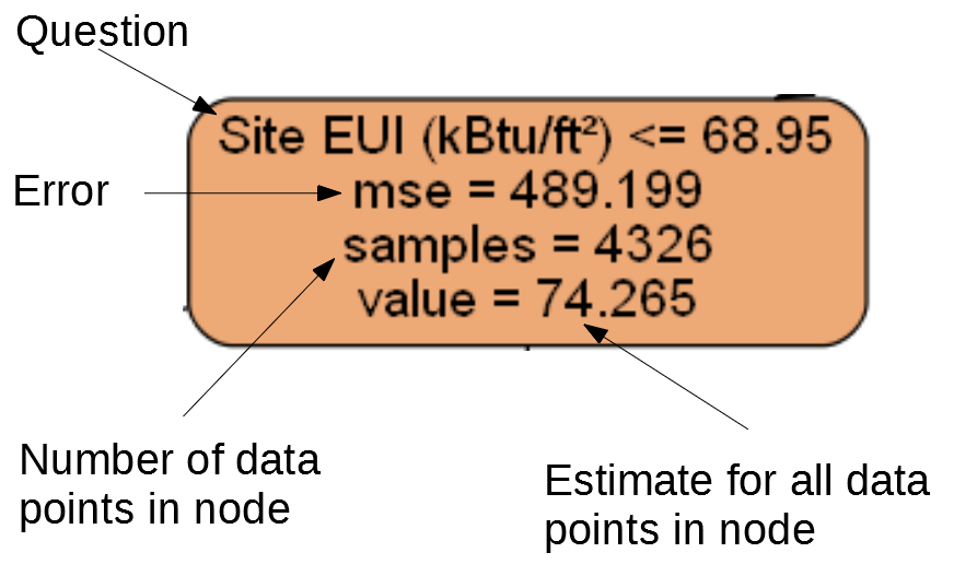Individual Node in Decision Tree

(Leaf nodes only have 2.–4. because they represent the final estimate and do not have any children).

A decision tree makes a prediction for a data point by starting at the top node, called the root, and working its way down through the tree. At each node, a yes-or-no question is asked of the data point. For example, the question for the node above is: Does the building have a Site EUI less than or equal to 68.95? If the answer is yes, the building is placed in the right child node, and if the answer is no, the building goes to the left child node.

This process is repeated at each layer of the tree until the data point is placed in a leaf node, at the bottom of the tree (the leaf nodes are cropped from the small tree image). The prediction for all the data points in a leaf node is the value. If there are multiple data points ( samples ) in a leaf node, they all get the same prediction. As the depth of the tree is increased, the error on the training set will decrease because there are more leaf nodes and the examples can be more finely divided. However, a tree that is too deep will overfit to the training data and will not be able to generalize to new testing data.

In the second article, we tuned a number of the model hyperparameters, which control aspects of each tree such as the maximum depth of the tree and the minimum number of samples required in a leaf node. These both have a significant impact on the balance of under vs over-fitting, and visualizing a single decision tree allows us to see how these settings work.

Although we cannot examine every tree in the model, looking at one lets us understand how each individual learner makes a prediction. This flowchart-based method seems much like how a human makes decisions, answering one question about a single value at a time. Decision-tree-based ensembles combine the predictions of many individual decision trees in order to create a more accurate model with less variance. Ensembles of trees tend to be very accurate, and also are intuitive to explain.

Local Interpretable Model-Agnostic Explanations (LIME)

The final tool we will explore for trying to understand how our model “thinks” is a new entry into the field of model explanations. LIME aims to explain a single prediction from any machine learning model by creating a approximation of the model locally near the data point using a simple model such as linear regression (the full details can be found in the paper ).

Here we will use LIME to examine a prediction the model gets completely wrong to see what it might tell us about why the model makes mistakes.

First we need to find the observation our model gets most wrong. We do this by training and predicting with the model and extracting the example on which the model has the greatest error:

**Prediction: 12.8615
Actual Value: 100.0000**

Next, we create the LIME explainer object passing it our training data, the mode, the training labels, and the names of the features in our data. Finally, we ask the explainer object to explain the wrong prediction, passing it the observation and the prediction function.

The plot explaining this prediction is below:

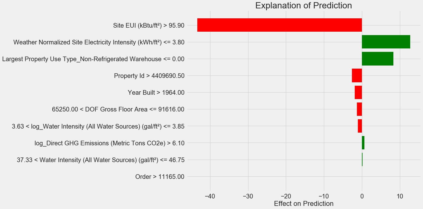Here’s how to interpret the plot: Each entry on the y-axis indicates one value of a variable and the red and green bars show the effect this value has on the prediction. For example, the top entry says the Site EUI is greater than 95.90 which subtracts about 40 points from the prediction. The second entry says the Weather Normalized Site Electricity Intensity is less than 3.80 which adds about 10 points to the prediction. The final prediction is an intercept term plus the sum of each of these individual contributions.

We can get another look at the same information by calling the explainer .show_in_notebook() method:

# Show the explanation in the Jupyter Notebook
exp.show_in_notebook()

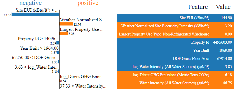Output from LIME Explainer Object

This shows the reasoning process of the model on the left by displaying the contributions of each variable to the prediction. The table on the right shows the actual values of the variables for the data point.

For this example, the model prediction was about 12 and the actual value was 100! While initially this prediction may be puzzling, looking at the explanation, we can see this was not an extreme guess, but a reasonable estimate given the values for the data point. The Site EUI was relatively high and we would expect the Energy Star Score to be low (because EUI is strongly negatively correlated with the score), a conclusion shared by our model. In this case, the logic was faulty because the building had a perfect score of 100.

It can be frustrating when a model is wrong, but explanations such as these help us to understand why the model is incorrect. Moreover, based on the explanation, we might want to investigate why the building has a perfect score despite such a high Site EUI. Perhaps we can learn something new about the problem that would have escaped us without investigating the model. Tools such as this are not perfect, but they go a long way towards helping us understand the model which in turn can allow us to make better decisions.

Documenting Work and Reporting Results

An often under-looked part of any technical project is documentation and reporting. We can do the best analysis in the world, but if we do not clearly communicate the results, then they will not have any impact!

When we document a data science project, we take all the versions of the data and code and package it so it our project can be reproduced or built on by other data scientists. It’s important to remember that code is read more often than it is written, and we want to make sure our work is understandable both for others and for ourselves if we come back to it a few months later. This means putting in helpful comments in the code and explaining your reasoning. I find Jupyter Notebooks to be a great tool for documentation because they allow for explanations and code one after the other.

Jupyter Notebooks can also be a good platform for communicating findings to others. Using notebook extensions, we can hide the code from our final report , because although it’s hard to believe, not everyone wants to see a bunch of Python code in a document!

Personally, I struggle with succinctly summarizing my work because I like to go through all the details. However, it’s important to understand your audience when you are presenting and tailor the message accordingly. With that in mind, here is my 30-second takeaway from the project:

1. Using the New York City energy data, it is possible to build a model that can predict the Energy Star Score of buildings to within 9.1 points.
2. The Site EUI and Weather Normalized Electricity Intensity are the most relevant factors for predicting the Energy Star Score.

Originally, I was given this project as a job-screening “assignment” by a start-up. For the final report, they wanted to see both my work and my conclusions, so I developed a Jupyter Notebook to turn in. However, instead of converting directly to PDF in Jupyter, I converted it to a Latex .tex file that I then edited in texStudio before rendering to a PDF for the final version. The default PDF output from Jupyter has a decent appearance, but it can be significantly improved with a few minutes of editing. Moreover, Latex is a powerful document preparation system and it’s good to know the basics.

At the end of the day, our work is only as valuable as the decisions it enables, and being able to present results is a crucial skill. Furthermore, by properly documenting work, we allow others to reproduce our results, give us feedback so we can become better data scientists, and build on our work for the future.

Conclusions

Throughout this series of posts, we’ve walked through a complete end-to-end machine learning project. We started by cleaning the data, moved into model building, and finally looked at how to interpret a machine learning model. As a reminder, the general structure of a machine learning project is below:

1. Data cleaning and formatting
2. Exploratory data analysis
3. Feature engineering and selection
4. Compare several machine learning models on a performance metric
5. Perform hyperparameter tuning on the best model
6. Evaluate the best model on the testing set
7. Interpret the model results to the extent possible
8. Draw conclusions and write a well-documented report

While the exact steps vary by project, and machine learning is often an iterative rather than linear process, this guide should serve you well as you tackle future machine learning projects. I hope this series has given you confidence to be able to implement your own machine learning solutions, but remember, none of us do this by ourselves! If you want any help, there are many incredibly supportive communities where you can look for advice.

A few resources I have found helpful throughout my learning process:

• Hands-On Machine Learning with Scikit-Learn and Tensorflow (Jupyter Notebooks for this book are available online for free)!
• An Introduction to Statistical Learning
• Kaggle: The Home of Data Science and Machine Learning
• Datacamp: Good beginner tutorials for practicing data science coding
• Coursera: Free and paid courses in many subjects
• Udacity: Paid programming and data science courses

As always, I welcome feedback and discussion and can be reached on Twitter @koehrsen_will.