
Machine Learning With Python On The Enron Dataset

##Investigating Fraud using Scikit-learn
Author’s Note: The following machine learning project was completed as part of the Udacity Data Analyst Nanodegree that I finished in May 2017. All of the code can be found on my GitHub repository for the class. I highly recommend the course to anyone interested in data analysis (that is anyone who wants to make sense of the mass amounts of data generated in our modern world) as well as to those who want to learn basic programming skills in an project-focused format.
Introduction
Dataset Background
The Enron email + financial dataset is a trove of information regarding the Enron Corporation, an energy, commodities, and services company that infamously went bankrupt in December 2001 as a result of fraudulent business practices. In the aftermath of the company’s collapse, the Federal Energy Regulatory Commission released more 1.6 million emails sent and received by Enron executives in the years from 2000–2002 (History of Enron). After numerous complaints regarding the sensitive nature of the emails, the FERC redacted a large portion of the emails, but about 0.5 million remain available to the public. The email + financial data contains the emails themselves, metadata about the emails such as number received by and sent from each individual, and financial information including salary and stock options. The Enron dataset has become a valuable training and testing ground for machine learning practicioners to try and develop models that can identify the persons of interests (POIs) from the features within the data. The persons of interest are the individuals who were eventually tried for fraud or criminal activity in the Enron investigation and include several top level executives. The objective of this project was to create a machine learning model that could separate out the POIs. I choose not to use the text contained within the emails as input for my classifier, but rather the metadata about the emails and the financial information. The ultimate objective of investigating the Enron dataset is to be able to predict cases of fraud or unsafe business practices far in advance, so those responsible can be punished, and those who are innocent are not harmed. Machine learning holds the promise of a world with no more Enrons, so let’s get started!
The Enron email + financial dataset, along with several provisional functions used in this report, is available on Udacity’s Machine Learning Engineer GitHub.
Outlier Investigation and Data Cleaning
The first step is to load in the all the data and scrutinize it for any errors that need to be corrected and outliers that should be removed. The data is provided in the form of a Python dictionary with each individual as a key and the information about the individual as values, and I will convert it to a pandas dataframe for easier data manipulation. I can then view the information about the dataset to see if anything stands out right away.
<class 'pandas.core.frame.DataFrame'>
Index: 146 entries, ALLEN PHILLIP K to YEAP SOON
Data columns (total 20 columns):
poi                          146 non-null bool
salary                       95 non-null float64
bonus                        82 non-null float64
long_term_incentive          66 non-null float64
deferred_income              49 non-null float64
deferral_payments            39 non-null float64
loan_advances                4 non-null float64
other                        93 non-null float64
expenses                     95 non-null float64
director_fees                17 non-null float64
total_payments               125 non-null float64
exercised_stock_options      102 non-null float64
restricted_stock             110 non-null float64
restricted_stock_deferred    18 non-null float64
total_stock_value            126 non-null float64
to_messages                  86 non-null float64
from_messages                86 non-null float64
from_poi_to_this_person      86 non-null float64
from_this_person_to_poi      86 non-null float64
shared_receipt_with_poi      86 non-null float64
dtypes: bool(1), float64(19)
memory usage: 23.0+ KB
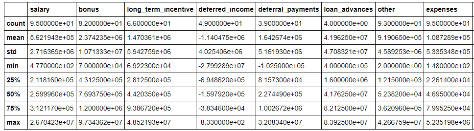
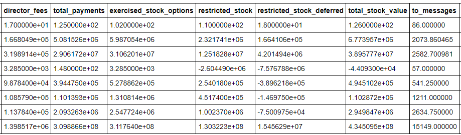
 From the info about the dataset, I can see that all the fields are floating point numbers except for the poi identification which is True/False. There are 146 rows in the dataframe which most likely mean there are 146 individuals’ information. Some of the maximum values seem unreasonable such the total payments which is $309 million or the to messages at 15,000! Those could be valid values, but they look suspicious on a first pass through the information.
Another observation is that there are numerous NaNs in both the email and financial fields. According to the official pdf documentation for the financial (payment and stock) data, values of NaN represent 0 and not unknown quantities. However, for the email data, NaNs are unknown information. Therefore, I will replace any financial data that is NaN with a 0 but will fill in the NaNs for the email data with the mean of the column grouped by person of interest. In other words, if a person has a NaN value for ‘to_messages’, and they are a person of interest, I will fill in that value with the mean value of ‘to_messages’ for a person of interest. If I chose to drop all NaNs, that would reduce the size of what is already a small dataset. As the quality of a machine learning model is proportional to the amount of data fed into it, I am hesitant to remove any information that could possibly be of use.
**from** **sklearn.preprocessing** **import** Imputer

_# Fill in the NaN payment and stock values with zero_
df[payment_data] = df[payment_data].fillna(0)
df[stock_data] = df[stock_data].fillna(0)

_# Fill in the NaN email data with the mean of column grouped by poi/ non_poi_
imp = Imputer(missing_values='NaN', strategy = 'mean', axis=0)

df_poi = df[df['poi'] == True];
df_nonpoi = df[df['poi']==False]

df_poi.ix[:, email_data] = imp.fit_transform(df_poi.ix[:,email_data]);
df_nonpoi.ix[:, email_data] = imp.fit_transform(df_nonpoi.ix[:,email_data]);
df = df_poi.append(df_nonpoi)
One simple way to check for outliers/incorrect data is to add up all of the payment related columns for each person and check if that is equal to the total payment recorded for the individual. I can also do the same for stock payments. If the data was entered by hand, I would expect that there may be a few errors that I can correct by comparing to the official PDF.
errors = (df[df[payment_data[:-1]].sum(axis='columns') != df['total_payments']])
errors
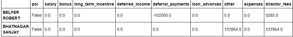
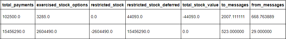
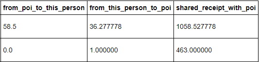 Sure enough, there are two individuals for which the sum of their payments does not add up to the recorded total payment. The errors appear to be caused by a misalignment of the columns; for Robert Belfer, the financial data has been shifted one column to the right, and for Sanjay Bhatnagar, the data has been shifted one column to the left. I can shift the columns to their correct positions and then check again to see if the individual payment and stock values add up to the respective totals.
_# Check for any more errors with the payment data_ len(df[df[payment_data[:-1]].sum(axis='columns') != df['total_payments']])

**Output:
0**

_# Check for any errors with the stock data_
len(df[df[stock_data[:-1]].sum(axis='columns') != df['total_stock_value']])

**Output:
0**
Correcting the shifted financial data eliminated two errors and there are not any more that are apparent from examination of the dataset. However, looking through the official financial PDF, I can see that I need to remove ‘TOTAL’ as it is currently the last row of the dataframe and it will throw off any predictions. (The total row is what was displaying the suspect maximum numbers in the summary of the dataframe.) Likewise, there is a row for ‘THE TRAVEL AGENCY IN THE PARK’, which according to the documentation, was a company co-owned by Enron’s former Chairman’s sister and is clearly not an individual that should be included in the dataset.
I can now look for outlying data points recorded in the different fields. I will try to be conservative in terms of removing the outliers because the dataset is rather small for machine learning in the first place. Moreover, the outliers might actually be important as they could represent patterns in the data that would aid in the identification of persons of interest. The official definition of a mild outlier is either below the (first quartile minus 1.5 times the Interquartile Range (IQR)) or above the (third quartile plus 1.5 times the IQR):
low outlier<first quartile−1.5 x IQR
high outlier>third quartile+1.5 * IQR
My approach will be to count the number of outlying features for each individual. I will then investigate the persons with the highest number of outliers to determine if they need to be removed.
IQR = df.quantile(q=0.75) - df.quantile(q=0.25)
first_quartile = df.quantile(q=0.25)
third_quartile = df.quantile(q=0.75)
outliers = df[(df>(third_quartile + 1.5*IQR) ) | (df<(first_quartile - 1.5*IQR) )].count(axis=1)
outliers.sort_values(axis=0, ascending=False, inplace=True)
outliers.head(12)

**Output:
LAY KENNETH L         15
FREVERT MARK A        12
BELDEN TIMOTHY N       9
SKILLING JEFFREY K     9
BAXTER JOHN C          8
LAVORATO JOHN J        8
DELAINEY DAVID W       7
KEAN STEVEN J          7
HAEDICKE MARK E        7
WHALLEY LAWRENCE G     7
RICE KENNETH D         6
KITCHEN LOUISE         6**
As this point, I need to do some research before blinding deleting outliers. Based on the small number of persons of interest initially in the dataset, I decided not to remove any individuals who are persons are interest regardless of their number of outliers. An outlier for a person of interest could be a sign of fradulent activity, such as evidence that someone is laundering illicit funds through the company payroll or is paying an accomplice to remain silent about illegal activity. I will manually examine several of the top outlying inviduals to see if I can glean any insights and to determine whom to remove.
A few interesting observations about the outliers:
- Kenneth Lay, the CEO of Enron from 1986–2001, presided over many of the illegal business activites and hence is one of the most vital persons of interest.
- Mark Frevert served as chief executive of Enron Europe from 1986–2000 and was appointed as chairman of Enron in 2001. He was a major player in the firm, although not a person of interest. I believe that he is not representative of the average employee at Enron during this time because of his substantial compensation and will remove him from the dataset.
- Timothy Belden was the former head of trading for Enron who developed the strategy to illegally raise energy prices in California. He was a person of interest and will definitely remain in the dataset.
- Jeffrey Skilling replaced Kenneth Lay as CEO of Enron in 2001 and orchestrated much of the fraud that destroyed Enron. As a person of interest, he will remain in the dataset.
- John Baxter was a former vice Enron vice chairman and died of an apparent self-inflicted gunshot before he was able to testify against other Enron executives. I will remove him from the dataset as he is not a person of interest.
- John Lavorato was a top executive in the energy-trading branch of Enron and received large bonuses to keep him from leaving Enron. As he was not a person of interest, and the large bonus ended up skewing his total pay, I think it would be appropriate to remove him from the dataset.
- Lawrence Whalley served as the president of Enron and fired Andrew Fastow once it was apparent the severity of Enron’s situation. He was investigated thoroughly but not identified as a person of interest and therefore will be removed from the dataset.
Total, I decided to remove four people from the dataset. I believe these removals are justified primarily because none of these individuals were persons of interest and they all were upper-level executives with pay levels far above the average employee. I do not think these top executives who did not commit fraud are indicative of the majority of employees at Enron who also did nothing illegal (i.e. they were not persons of interest).
_# Remove the outlier individuals_
df.drop(axis=0, labels=['FREVERT MARK A', 'LAVORATO JOHN J', 'WHALLEY LAWRENCE G', 'BAXTER JOHN C'], inplace=True)

_# Find the number of poi and non poi now in the data_
df['poi'].value_counts()

**Output:
False    122
True      18**
There are a total of 2800 observations of financial and email data in the set now that the data cleaning has been finished. Of these, 1150 or 41% are 0 for financial (payment and stock) values. There are 18 persons of interest, comprising 12.9% of the individuals.
Initial Algorithm Training and Performance Metrics
The first training and testing I will do will be on all of the initial features in the dataset. This is in order to gauge the importance of the features and to serve a baseline to observe the performance before any feature selection or parameter tuning. The four algorithms I have selected for initial testing are Gaussian Naive Bayes (GaussianNB), DecisionTreeClassifier, Support Vector Classifier (SVC), and KMeans Clustering. I will run the algorithms with the default parameters except I will alter the kernel used in the Support Vector Machine to be linear and I will select number of clusters = 2 for KMeans as I know in advance that the targets are only two categories that should be classified. Although accuracy would appear to be the obvious choice for evaluating the quality of a classifier, accuracy can be a crude measure at times, and is not suited for some datasets including the Enron one. For example, if a classifier were to guess that all of the samples in the cleaned dataset were not persons of interest, it would have an accuracy of 87.1%. However, this clearly would not satisfy the objective of this investigation which is to create a classifier that can identify persons of interest. Therefore, different metrics are needed to evaluate the classifiers to to gauge performance. The two selected for use in this project are Precision and Recall.
- Precision is the number of correct positive classifications divided by the total number of positive labels assigned. In other words, it is the fraction of persons of interest predicted by the algorithm that are truly persons of interest. Mathematically precision is defined as
precision=true positives / (true positives+false positives)
- Recall is the number of correct positive classifications divided by the number of positive instances that should have been identified. In other words, it is the fraction of the total number of persons of interestin the data that the classifier identifies. Mathematically, recall is defined as
recall=true positives / (true positives+false negatives)
Precision is also known as positive predictive value while recall is called the sensitivity of the classifier. A combined measured of precision and recall is the F1 score. Is it the harmonic mean of precision and recall. Mathematically, the F1 score is defined as:
F1 Score=2 (precision x recall) / (precision+recall)
For this project, the objective was a precision and a recall both greater than 0.3. However, I believe it is possible to do much better than that with the right feature selection and algorithm tuning. For the majority of my tuning and optimization using GridSearchCV, I will use the F1 score because it takes into account both the precision and recall.
Scaling
Initial Algorithm Training and Performance Metrics
The first training and testing I will do will be on all of the initial features in the dataset. This is in order to gauge the importance of the features and to serve a baseline to observe the performance before any feature selection or parameter tuning. The four algorithms I have selected for initial testing are Gaussian Naive Bayes (GaussianNB), DecisionTreeClassifier, Support Vector Classifier (SVC), and KMeans Clustering. I will run the algorithms with the default parameters except I will alter the kernel used in the Support Vector Machine to be linear and I will select number of clusters = 2 for KMeans as I know in advance that the targets are only two categories that should be classified. Although accuracy would appear to be the obvious choice for evaluating the quality of a classifier, accuracy can be a crude measure at times, and is not suited for some datasets including the Enron one. For example, if a classifier were to guess that all of the samples in the cleaned dataset were not persons of interest, it would have an accuracy of 87.1%. However, this clearly would not satisfy the objective of this investigation which is to create a classifier that can identify persons of interest. Therefore, different metrics are needed to evaluate the classifiers to to gauge performance. The two selected for use in this project are Precision and Recall.
- Precision is the number of correct positive classifications divided by the total number of positive labels assigned. In other words, it is the fraction of persons of interest predicted by the algorithm that are truly persons of interest. Mathematically precision is defined as
precision=true positivestrue positives+false positivesprecision=true positivestrue positives+false positives
- Recall is the number of correct positive classifications divided by the number of positive instances that should have been identified. In other words, it is the fraction of the total number of persons of interestin the data that the classifier identifies. Mathematically, recall is defined as
recall=true positivestrue positives+false negativesrecall=true positivestrue positives+false negatives
Precision is also known as positive predictive value while recall is called the sensitivity of the classifier. A combined measured of precision and recall is the F1 score. Is it the harmonic mean of precision and recall. Mathematically, the F1 score is defined as:
F1 Score=2 (precision x recall)precision+recallF1 Score=2 (precision x recall)precision+recall
For this project, the objective was a precision and a recall both greater than 0.3. However, I believe it is possible to do much better than that with the right feature selection and algorithm tuning. For the majority of my tuning and optimization using GridSearchCV, I will use the F1 score because it takes into account both the precision and recall.
Scaling
The only data preparation I will do for initial testing of the algorithms is to scale the data such that it has a zero mean and a unit variance. This process is called normalization and is accomplished using the scale function from the sklearn preprocessing module. Scaling of some form (whether that is MinMax scaling or normalization) is usually necessary because there are different units for the features in the dataset. Scaling creates non-dimensional features so that those features with larger units do not have an undue influence on the classifier as would be the case if the classifier uses some sort of distance measurement (such as Euclidean distance) as a similarity metric. Here is a good dicussion of feature scaling and normalization.
**from** **sklearn.preprocessing** **import** scale
**from** **sklearn.naive_bayes** **import** GaussianNB
**from** **sklearn.tree** **import** DecisionTreeClassifier
**from** **sklearn.svm** **import** SVC
**from** **sklearn.cluster** **import** KMeans
**from** **sklearn.ensemble** **import** AdaBoostClassifier
**import** **tester**

_# Scale the dataset and send it back to a dictionary_
scaled_df = df.copy()
scaled_df.ix[:,1:] = scale(scaled_df.ix[:,1:])
my_dataset = scaled_df.to_dict(orient='index')

_# Create and test the Gaussian Naive Bayes Classifier_
clf = GaussianNB()
tester.dump_classifier_and_data(clf, my_dataset, features_list)
tester.main();

_# Create and test the Decision Tree Classifier_
clf = DecisionTreeClassifier()
tester.dump_classifier_and_data(clf, my_dataset, features_list)
tester.main();

_# Create and test the Support Vector Classifier_
clf = SVC(kernel='linear')
tester.dump_classifier_and_data(clf, my_dataset, features_list)
tester.main()

_# Create and test the K Means clustering classifier_
clf = KMeans(n_clusters=2)
tester.dump_classifier_and_data(clf, my_dataset, features_list)
tester.main();
The results from running the four classifiers on the entire original featureset with no parameter tuning are summarized in the table below
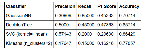 From the first run through the four algorithms, I can see that the decision tree performed best, followed by the gaussian naive bayes, support vector machine, and Kmeans clustering. In fact, the decision tree and naive Bayes classifiers both perform well enough to meet the standards for the project. Nonetheless, there is much work that can be done to improve these metrics.
A Quick Note on Validation
The validation strategy used here is a form of cross-validation that is implemented in the provided tester.py script. Cross-validation performs multiple splits on the dataset and in each split, forms a different training and testing set. Each iteration, the classifier is fit on a training set and then tested on a testing set. The next iteration the classifier is again trained and tested, but on different sets and this process continues for the number of splits made of the dataset. Cross-validation prevents one from making the classic mistake of training an algoithm on the same data used to test the algorithm. If this happens, the test results may show that the classifier is accurate, but that is only because the algorithm has seen the testing data before. When the classifier is deployed on novel samples (implemented in the real world), the performance may be poor because it was trained and tuned for a very specific set of instances. The classifier will not be able to generalize to new cases becuase it is only fit and tuned to the specific samples it is tested on. Cross-validation solves this issue by training and testing on multiple different subsets of the features and labels and is ideal for use on small datasets to avoid overfitting. Throughout my analysis, I used cross-validation to assess the performance of my algorithms. The tester.py script uses the StratifiedShuffleSplit cross-validation method, and GridSearchCV, which is used to find the optimal number of features and the best parameters, employs cross validation with the StratifiedKFolds cross-validator. In both cases, the dataset is split 10 times into training and testing sets.
Feature Engineering
The next step is to create new features from the existing information that could possibly improve performance. I will also need to carry out feature selection to remove those features that are not useful for predicting a person of interest.
After thinking about the background of the Enron case and the information to work with contained in the dataset, I decided on three new features to create from the email metadata. The first will be the ratio of emails to an individual from a person of interest to all emails addressed to that person, the second is the same but for messages to persons of interest, and the third will be the ratio of email receipts shared with a person of interest to all emails addressed to that individual. The rational behind these choices is that the absolute number of emails from or to a person of interest might not matter so much as the relative number considering the total emails an individual sends or receives. My instinct says that individuals who interact more with a person of interest (as indicated by emails) are themselves more likely to be a person of interest because the fraud was not perpertrated alone and required a net of persons. However, there are also some innocent persons who may have sent or received many emails from persons of interest simply in the course of their daily and perfectly above-the-table work.
_# Add the new email features to the dataframe_
df['to_poi_ratio'] = df['from_poi_to_this_person'] / df['to_messages']
df['from_poi_ratio'] = df['from_this_person_to_poi'] / df['from_messages']
df['shared_poi_ratio'] = df['shared_receipt_with_poi'] / df['to_messages']
At this point I will also create new features using the financial data. I have a few theories that I formed from my initial data exploration and reading about the Enron case. I think that people recieving large bonuses may be more likely to be persons of interest becuase the bonuses could be a result of fraudulent activity. It would be easier to pass off illegal funds as a bonus rather than a salary raise which usually involves a contract and input from shareholders. The two new features will be the bonus in relation to the salary, and the bonus in relation to total payments. There are now a total of 25 features, some of which are most likely redudant or not of any value. I will perform feature reduction/selection to optimize the number of features so I am not worried about the initial large number of features. Moreover, the algorithms I am using are able to train relatively quickly even with the large number of features because the total number of data samples is small.
_# Create the new financial features and add to the dataframe_
df['bonus_to_salary'] = df['bonus'] / df['salary']
df['bonus_to_total'] = df['bonus'] / df['total_payments']
After adding in the features, the results for all of the algorithms have improved and are summarized below:
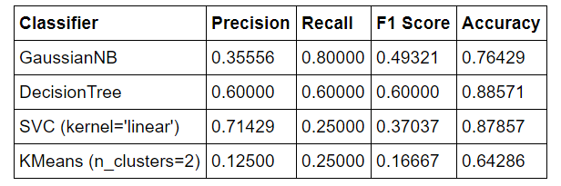 The F1 score for the decision tree is stil the highest followed by the Gaussian Naive Bayes Classifier. At this point, neither the SVC with the linear kernel nor the KMeans clustering pass the standards of 0.3 for precision and recall. I will drop the latter two algorithms and I will also drop the GaussianNB in favor of the AdaBoost Classifier because I want to experiment with tunable parameters and GaussianNB does not have any. AdaBoost takes a weak classifier, and trains it multiple times on a dataset, each run adjusting the weights of incorrectly classified instances to concentrate on the most difficult to classify samples. AdaBoost therefore works to iteratively improve an existing classifier and can be used in conjuction with a DecisionTree or GaussianNB.
Feature Visualization
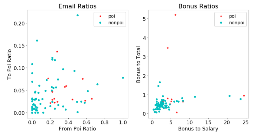
In order to understand the features I have, I want to visualize at least some of the data. Visualizing the data can help with feature selection by revealing trends in the data. The following is a simple scatterplot of the email ratio features I created and the bonus ratios I created. For the email ratios, my intuition tells me that persons of interest would tend to have points higher in both ratios and therefore should tend to be located in the upper right of the plot. For the bonus ratios, I would expect similar behavior. In both plots, the non persons of interest are clustered to the bottom left, but there is not a clear trend among the persons of interest. I also noticed suspiciously that several of the bonus to total ratios are greater than one. I thought this might be an error in the dataset, but after looking at the official financial data document, I saw some individuals did indeed have larger bonuses than their total payments because they had negative values in other payment categories. There are no firm conclusions to draw from these graphs, but it does appear that the new features might be of some use in identifiying persons of interest as the POIs exhibit noticeable differences from the non POIs in both graphs.
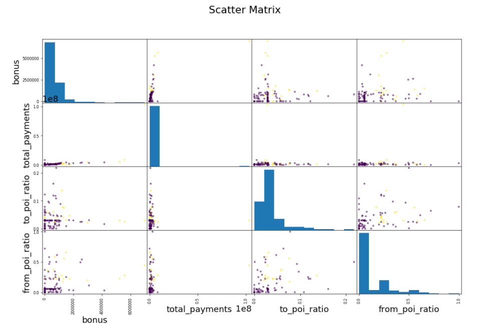
 The plot below is a scatter matrix showing all the relationships between four selected features: ‘bonus’, ‘total_payments’, ‘to_poi_ratio’, and ‘from_poi_ratio’. The diagonals are histograms because a variable correlated with itself is simply one. The persons of interest are plotted in yellow and the non persons of interest are the purple points. Overall, there do seem to be a couple of trends. Looking at the bonus vs from_poi_ratio, the persons of interest tend to be further to the right and higher than non persons of interest. This indicates that persons of interest tend to recieve larger bonuses and they send more emails to other persons of interest. The scale on the total payments graph makes those graphs somewhat difficult to read but it can be seen that persons of interest tend to also have higher total payments. This trend can be seen in the to_poi_ratio vs total_payments scatter plot. Perhaps this demonstrates that persons of interest recieve more total payments due to fraudulent activity or because they tend to be employed at an upper level in the company and therefore command higher salaries.
Overall, the visualizations do not offer many clear trends. However, it is still important to get a feel for the scale of the data and to check and see if there are any patterns evident that could inform the creation of new features or the selection of existing features. A great visualization of the Enron email and financial dataset is available as a navigable dashboard.
 # Feature Selection
There are several methods available for performing feature selection in machine learning. One is simply to look at the feature importances for a classifier and modify the list of features to exclude those with an importance below a chosen threshold. Another is to use SelectKBest and have the k-best features, defined by the amount of variance explained, automatically selected for use in the classifier. I will look at the feature importances for both the DecisionTree and the AdaBoost Classifier, but I would prefer to use SelectKBest to actually choose the features to keep. Additionally, I can use GridSearchCV in combination with SelectKBest to find the optimal number of features to use. This will run through a number of k values and choose the one that yields the highest value according to a designated performance metric.
First, I will manually look at the feature importances for both classifiers to get a sense of which features are most important. One of the neat aspects about machine learning is that it can help humans to think smarter. By looking at what the algorithm chooses as the most important features to identify persons of interest, it can inform humans what they should be looking for in similar cases. (One example of this in the real world is when Google’s AlphaGo defeated Lee Sedol in Go, it advanced the entire state of Go by providing new insights and strategies into a game humans have played for millenia.)
_# Get the feature importances of the DecisionTree Classifier_
tree_feature_importances = (clf_tree.feature_importances_)
tree_features = zip(tree_feature_importances, features_list[1:])
tree_features = sorted(tree_features, key= **lambda** x:x[0], reverse=True)

_# Display the feature names and importance values_
**print**('Tree Feature Importances:**\n**')
**for** i **in** range(10):
    **print**('{} : {:.4f}'.format(tree_features[i][1], tree_features[i][0]))

**Output:** Tree Feature Importances:

**from_poi_ratio : 0.3782
shared_receipt_with_poi : 0.2485
expenses : 0.2476
shared_poi_ratio : 0.0665
from_poi_to_this_person : 0.0592
salary : 0.0000
bonus : 0.0000
long_term_incentive : 0.0000
deferred_income : 0.0000
deferral_payments : 0.0000**
Find the feature importances for the AdaBoost Classifier
_# Get the feature importances for the AdaBoost Classifier_
ada_feature_importances = clf_ada.feature_importances_
ada_features = zip(ada_feature_importances, features_list[1:])

_# Display the feature names and importance values_
**print**('Ada Boost Feature Importances:**\n**')
ada_features = sorted(ada_features, key=**lambda** x:x[0], reverse=True)
**for** i **in** range(10):
    **print**('{} : {:.4f}'.format(ada_features[i][1], ada_features[i][0]))

**Output:
Ada Boost Feature Importances:

shared_receipt_with_poi : 0.1200
exercised_stock_options : 0.1000
from_this_person_to_poi : 0.1000
to_poi_ratio : 0.1000
deferred_income : 0.0800
from_messages : 0.0800
from_poi_ratio : 0.0800
other : 0.0600
total_stock_value : 0.0600
shared_poi_ratio : 0.0400**
It is interesting to compare the feature importances for the DecisionTree and the AdaBoost classifiers. The top 10 features are not in close agreement even though both classifiers achieve a respectable F1 Score greater than 0.5. However, rather than manually selecting the features to keep, I will use GridSearchCV with SelectKBest to find the optimal number of features for the classifiers. GridSearchCV runs through a parameter grid and tests all the different configurations provided to it. It returns the parameters that yield the maximum score. I will use a scoring parameter of F1 because that is what I would like to maximize, and a cross-validation with 10 splits to ensure that I am not overfitting the algorithm to the training data.
**from** **sklearn.model_selection** **import** GridSearchCV

n_features = np.arange(1, len(features_list))

_# Create a pipeline with feature selection and classification_
pipe = Pipeline([
    ('select_features', SelectKBest()),
    ('classify', DecisionTreeClassifier())
])

param_grid = [
    {
        'select_features__k': n_features
    }
]

_# Use GridSearchCV to automate the process of finding the optimal number of features_
tree_clf= GridSearchCV(pipe, param_grid=param_grid, scoring='f1', cv = 10)
tree_clf.fit(features, labels);
According to the grid search performed with SelectKBest with the number of features ranging from 1 to 24 (the number of features minus one), the optimal number of features for the decision tree classifier is 19. I can look at the scores assigned to the top performing features using the scores attribute of SelectKBest.
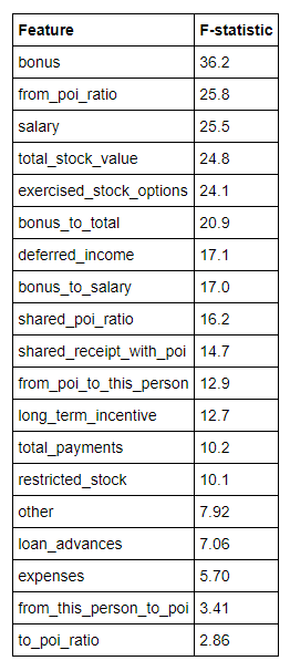
SelectKBest defaults to scoring parameters using the ANOVA F-value which is a measure of variation between sample means. It describes how much of the variance between labels is explained by a particular feature. A higher value therefore means that there is more variation in that feature between person of interests and non persons of interest. The following table summarizes the Decision Tree features and the ANOVA F-Value returned by SelectKBest with k = 19. These are the features I used in my final DecisionTreeClassifier.
 Running the DecisionTreeClassifier with SelectKMeans and k = 19 yields an F1 score of 0.700. I very pleased with that result and have decided on the 19 features I will use with the DecisionTreeClassifier. Any further improvement from this classifier will come in the parameter tuning section of the investigation.
A similar procedure with GridSearchCV and SelectKBest will be carried out to determine the optimal number of features to use with the AdaBoostClassifier.
n_features = np.arange(1, len(features_list))
_# Create a pipeline of feature selection and classifier_
pipe = Pipeline([
    ('select_features', SelectKBest()),
    ('classify', AdaBoostClassifier())
])

param_grid = [
    {
        'select_features__k': n_features
    }
]

_# Use GridSearchCV to automate the process of finding the optimal number of features_
ada_clf= GridSearchCV(pipe, param_grid=param_grid, scoring='f1', cv =10)
ada_clf.fit(features, labels)
The ideal number of parameters for SelectKMeans using GridSearch for the AdaBoostClassifier was 23. This resulted in a slightly lower F1 score of 0.689 and I will use the 23 highest scoring features with the AdaBoostClassifier. The F-Scores are the same so I will not show them all again.
At this point I could also perform Principal Component Analysis to further reduce the number of features, but I think that the performance I am seeing does not necessitate the use of PCA, and the algorithms do not take very long to train even on a large number of features. PCA creates new features by selecting dimensions of the data with the greatest variation even in these features do not necessarily represent actual quantifiable values in the dataset. I prefer the idea that I know exactly all the features I am putting into the model if that is possible. This is one way that I try to combat the black box problem in machine learning. If I at least know what is going in to a model, then I can try to understand why the model returned a certain classification and it can inform my thinking to enable me to create smarter machine learning classifiers in the future.
Hyperparameter Optimization
Parameter tuning is the process of optimizing the “settings” of a machine learning algorithm to achieve maximum performance on a given dataset. A machine learning algorithm is simply a sequence of rules that is applied to a set of features by a computer in order to arrive at a classification. Parameter tuning can be thought of as iteratively altering these rules to produce better classifications. Sci-kit learn implements default parameters for each algorithm designed to get a classifier up and running by generalizing to as many datasets as possible with decent performance. However, it is possible to achieve greater performance by changing these algorithm parameters (although they are often used interchangeably, technically ‘hyperparameters’ are aspects of the estimator that must be set beforehand by the user while the model ‘parameters’ are learned from the dataset; see here for a discussion). The proces of parameter tuning for a dataset can either by carried out manually, by selecting different configurations, performing cross-validation, and selecting the settings that return the highest performance, or it can be automated by another algorithm such as GridSearchCV. A parameter grid is passed to GridSearchCV that consists of a number of combinations of parameters to test with an algorithm, and the search returns the parameters that maximize performance. The parameters available for an algorithm in sci-kit learn can be found in the classifier documentation. My process for algorithm tuning will be to examine the sci-kit learn documentation, construct a parameter grid with a wide range of configurations, and use GridSearchCV to find the optimal settings.
The decision tree will be up first. Looking at the sci-kit learn documentation for the DecisionTreeClassifier, there are numerous parameters that can be changed, each of which alter the manner in which the algorithm makes decisions as it parses the features and creates the ‘tree’. For example, criterion can either be set as ‘gini’ or ‘entropy’ which determines how the algorithm measures the quality of a split of a node, or in other words, which branch of the tree to take to arrive at the correct classification. (‘gini’ utilizies the gini impurity while ‘entropy’ maximizes the [information gain] at each branching(https://en.wikipedia.org/wiki/Information_gain_ratio). I will put both options in my parameter grid and let grid search determine which is the best. The other three parameters I will tune are min_samples_split, max_depth, and max_features. GridSearch will be directed by cross-validation with 10 splits of the data, and the scoring criteria is specified as F1 because that is the primary measure of classifier performance I used to account for both precision and recall.
_# Create a pipeline with feature selection and classifier_
tree_pipe = Pipeline([
    ('select_features', SelectKBest(k=19)),
    ('classify', DecisionTreeClassifier()),
])

_# Define the configuration of parameters to test with the_
_# Decision Tree Classifier_
param_grid = dict(classify__criterion = ['gini', 'entropy'] ,
                  classify__min_samples_split = [2, 4, 6, 8, 10, 20],
                  classify__max_depth = [None, 5, 10, 15, 20],
                  classify__max_features = [None, 'sqrt', 'log2', 'auto'])

_# Use GridSearchCV to find the optimal hyperparameters for the classifier_
tree_clf = GridSearchCV(tree_pipe, param_grid = param_grid, scoring='f1', cv=10)
tree_clf.fit(features, labels)

_# Get the best algorithm hyperparameters for the Decision Tree_
tree_clf.best_params_

**Output:
{'classify__criterion': 'entropy',
 'classify__max_depth': None,
 'classify__max_features': None,
 'classify__min_samples_split': 20}**
The best parameters identified are shown above. Using GridSearch saved me from the tedious taask of running through and manually evaluating all of the combinations of hyperparameters. I will now implement the best parameters and assess the Decision Tree Classifier using the cross validation available in the tester.py function.
_# Create the classifier with the optimal hyperparameters as found by GridSearchCV_
tree_clf = Pipeline([
    ('select_features', SelectKBest(k=20)),
    ('classify', DecisionTreeClassifier(criterion='entropy', max_depth=None, max_features=None, min_samples_split=20))
])

_# Test the classifier using tester.py_
tester.dump_classifier_and_data(tree_clf, my_dataset, features_list)
tester.main()
According to the cross validation in tester.py, my F1 score is around 0.800 with the optimal parameters. I am satisfied with the recall and precision score of the DecisionTreeClassifier but I will try the AdaBoostClassifier using the same approach because I am curious to see if I can beat the F1 score.
It’s time to look at the Sci-kit learn documentation for the AdaBoost Classifier to see the parameters available to tune. The AdaBoostClassifier boosts another ‘base’ classifier, which by default is the Decision Tree. I can alter this using the base_estimator parameter to test out a random forest and the gaussian naive bayes classification. The other parameters I can change are n_estimators which is how many weak models to fit and learning_rate, a measure of the weight given to each classifier. AdaBoost is generally used on weak classifiers, or those that perform only slightly better than random. One example would be a decision stump or a decision tree with only a single layer. In theory, the AdaBoost Classifier should perform better than the decision tree because it runs the decision tree multiple times and iteratively adjusts the weights given to each featureto make more accurate predictions. However, in practice, a more complex algorithm does not always perform better than a simple model and, at the end of the day, more quality data will beat a highly tuned algorithm.
_# Create the pipeline with feature selection and AdaBoostClassifier_
ada_pipe = Pipeline([('select_features', SelectKBest(k=20)),
                     ('classify', AdaBoostClassifier())
                    ])

_# Define the parameter configurations to test with GridSearchCV_
param_grid = dict(classify__base_estimator=[DecisionTreeClassifier(), RandomForestClassifier(), GaussianNB()],
                  classify__n_estimators = [30, 50, 70, 120],
                  classify__learning_rate = [0.5, 1, 1.5, 2, 4])

_# Use GridSearchCV to automate the process of finding the optimal parameters_
ada_clf = GridSearchCV(ada_pipe, param_grid=param_grid, scoring='f1', cv=10)
ada_clf.fit(features, labels)

_# Display the best parameters for the AdaBoostClassifier_
ada_clf.best_params_

**Output:
{'classify__base_estimator': DecisionTreeClassifier(class_weight=None, criterion='gini', max_depth=None,
             max_features=None, max_leaf_nodes=None,
             min_impurity_split=1e-07, min_samples_leaf=1,
             min_samples_split=2, min_weight_fraction_leaf=0.0,
             presort=False, random_state=None, splitter='best'),
 'classify__learning_rate': 1,
 'classify__n_estimators': 70}**
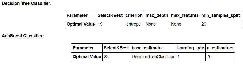
Here is a brief summary of the results using GridSearch for feature selection and then for algorithm tuning.
 # Results
_# Implement the Decision Tree Classifier with the optimal parameters_
tree_clf = Pipeline([
    ('select_features', SelectKBest(k=19)),
    ('classify', DecisionTreeClassifier(criterion='entropy', max_depth=None, max_features=None, min_samples_split=20))
])

_# Test the classifier with cross-validation_
tester.dump_classifier_and_data(tree_clf, my_dataset, features_list)
tester.main()

_# Implement the AdaBoost Classifier with the optimal parameters_
ada_clf = Pipeline([('select_features', SelectKBest(k=23)),
                   ('classify', AdaBoostClassifier(base_estimator=DecisionTreeClassifier(), learning_rate=1, n_estimators=70))
                   ])

_# Test the classifier with cross-validation_
tester.dump_classifier_and_data(ada_clf, my_dataset, features_list)
tester.main()
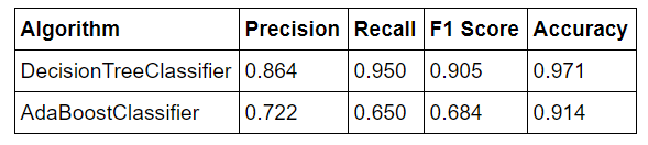
The results from running the final versions of the algorithms are shown below:
 # Conclusion
Although the script I used to test the classifier implemented cross-validation, I was skeptical of the relatively high precision, recall, and F1 score recorded. I was conscious that I had somehow overfit my model to the data even though the script implements cross-validation. Looking through the tester.py script, I saw that the random seed for the cross-validation split was set at 42 in order to generate reproducible results. I changed the random seed and sure enough, the performance of my model decreased. Therefore, I must have made the classic mistake of overfitting on my training set for the given cross-validation random seed, and I will need to look out for this problem in the future. Even taking precuations against overfitting, I had still optimized my model for a specific set of data. In order to get a better indicator of the perfomance of the Decision Tree model, I ran 10 tests with different random seeds and found the average performance metrics. The final results for my model are summarized below:
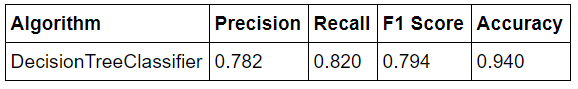 The results are still relatively high given the nature of the persons of interest identification task, but not as questionably high as testing with a single random split of the data. Due to the small size of the available data, even a minor change such as altering the random seed when doing a train-test split can have significant effects on the performance of the algorithm which must be accounted for by testing over many subsets and calculating the average performance.
A precision score of 0.782 means that of the individuals labeled by my model as persons of interest, 78.2% of them were indeed persons of interest. A recall score of 0.820 means that my model identified 82.0% of persons of interest present in the entire dataset.
The main takeaway from this project was the important of quality data as compared to fine-tuning the algorithm. Feature engineering, through the creation of new features and the selection of those with the greatest explained variance, increased the F1 score of the classifier from ~ 0.40 to ~ 0.70. However, tuning the hyperparameters of the algorithm only increased the F1 score to 0.80. Subsequently, when developing future machine learning models, I will focus on collecting as much high-quality data as I can before I even think about training and tuning the algorithm. This point was elucidated in a 2009 paper from Alon Halevy and Peter Norvig titled “The Unreasonable Effectiveness of Data.” The main argument of the paper is that as the amount of valid data increases, the choice of algorithm matters less and less and even the simplest algorithm can match the performance of the most highly tuned algorithm. Moreover, this project showed me that human intuition about a situation will not always match the results returned by a machine learning model. For example, Imy hypothesis was that the most highly predictive indicators of fradulent activity would be emails to/from persons of interest. Using automatic feature selection showed that the order of importance was bonus, from_poi_ratio, salary, total_stock_value. My intuition was partly correct, but the algorithm also had other (and more accurate) ideas for what mattered when it came to identifying persons of interest. Nonetheless, this discrepancy between my thinking and the classifier provides a chance to learn from the machine and update my mindset. Ultimately, I see the importance of machine learning not in outsourcing all decisions to algorithms, but in using machines to process and provide insights from data that can inform smarter thinking and enable humans to create more efficient systems.\
Appendix
tester.py Provisional Function provided by Udacity.
"" a basic script for importing student's POI identifier,
    and checking the results that they get from it

    requires that the algorithm, dataset, and features list
    be written to my_classifier.pkl, my_dataset.pkl, and
    my_feature_list.pkl, respectively
    that process should happen at the end of poi_id.py
"""

import pickle
import sys
from sklearn.cross_validation import StratifiedShuffleSplit
sys.path.append("../tools/")
from feature_format import featureFormat, targetFeatureSplit

PERF_FORMAT_STRING = "\
\tAccuracy: {:>0.{display_precision}f}\tPrecision: {:>0.{display_precision}f}\t\
Recall: {:>0.{display_precision}f}\tF1: {:>0.{display_precision}f}\tF2: {:>0.{display_precision}f}"
RESULTS_FORMAT_STRING = "\tTotal predictions: {:4d}\tTrue positives: {:4d}\tFalse positives: {:4d}\
\tFalse negatives: {:4d}\tTrue negatives: {:4d}"

def test_classifier(clf, dataset, feature_list, folds = 1000):
    data = featureFormat(dataset, feature_list, sort_keys = True)
    labels, features = targetFeatureSplit(data)
    cv = StratifiedShuffleSplit(labels, folds, random_state = 42)
    true_negatives = 0
    false_negatives = 0
    true_positives = 0
    false_positives = 0
    for train_idx, test_idx in cv:
        features_train = []
        features_test  = []
        labels_train   = []
        labels_test    = []
        for ii in train_idx:
            features_train.append( features[ii] )
            labels_train.append( labels[ii] )
        for jj in test_idx:
            features_test.append( features[jj] )
            labels_test.append( labels[jj] )

        ### fit the classifier using training set, and test on test set
        clf.fit(features_train, labels_train)
        predictions = clf.predict(features_test)
        for prediction, truth in zip(predictions, labels_test):
            if prediction == 0 and truth == 0:
                true_negatives += 1
            elif prediction == 0 and truth == 1:
                false_negatives += 1
            elif prediction == 1 and truth == 0:
                false_positives += 1
            elif prediction == 1 and truth == 1:
                true_positives += 1
            else:
                print "Warning: Found a predicted label not == 0 or 1."
                print "All predictions should take value 0 or 1."
                print "Evaluating performance for processed predictions:"
                break
    try:
        total_predictions = true_negatives + false_negatives + false_positives + true_positives
        accuracy = 1.0*(true_positives + true_negatives)/total_predictions
        precision = 1.0*true_positives/(true_positives+false_positives)
        recall = 1.0*true_positives/(true_positives+false_negatives)
        f1 = 2.0 * true_positives/(2*true_positives + false_positives+false_negatives)
        f2 = (1+2.0*2.0) * precision*recall/(4*precision + recall)
        print clf
        print PERF_FORMAT_STRING.format(accuracy, precision, recall, f1, f2, display_precision = 5)
        print RESULTS_FORMAT_STRING.format(total_predictions, true_positives, false_positives, false_negatives, true_negatives)
        print ""
    except:
        print "Got a divide by zero when trying out:", clf
        print "Precision or recall may be undefined due to a lack of true positive predicitons."

CLF_PICKLE_FILENAME = "my_classifier.pkl"
DATASET_PICKLE_FILENAME = "my_dataset.pkl"
FEATURE_LIST_FILENAME = "my_feature_list.pkl"

def dump_classifier_and_data(clf, dataset, feature_list):
    with open(CLF_PICKLE_FILENAME, "w") as clf_outfile:
        pickle.dump(clf, clf_outfile)
    with open(DATASET_PICKLE_FILENAME, "w") as dataset_outfile:
        pickle.dump(dataset, dataset_outfile)
    with open(FEATURE_LIST_FILENAME, "w") as featurelist_outfile:
        pickle.dump(feature_list, featurelist_outfile)

def load_classifier_and_data():
    with open(CLF_PICKLE_FILENAME, "r") as clf_infile:
        clf = pickle.load(clf_infile)
    with open(DATASET_PICKLE_FILENAME, "r") as dataset_infile:
        dataset = pickle.load(dataset_infile)
    with open(FEATURE_LIST_FILENAME, "r") as featurelist_infile:
        feature_list = pickle.load(featurelist_infile)
    return clf, dataset, feature_list

def main():
    ### load up student's classifier, dataset, and feature_list
    clf, dataset, feature_list = load_classifier_and_data()
    ### Run testing script
    test_classifier(clf, dataset, feature_list)

if __name__ == '__main__':
    main()