
An Implementation and Explanation of the Random Forest in Python
A guide for using and understanding the random forest by building up from a single decision tree.
Fortunately, with libraries such as Scikit-Learn, it’s now easy to implement hundreds of machine learning algorithms in Python. It’s so easy that we often don’t need any underlying knowledge of how the model works in order to use it. While knowing all the details is not necessary, it’s still helpful to have an idea of how a machine learning model works under the hood. This lets us diagnose the model when it’s underperforming or explain how it makes decisions, which is crucial if we want to convince others to trust our models.
In this article, we’ll look at how to build and use the Random Forest in Python. In addition to seeing the code, we’ll try to get an understanding of how this model works. Because a random forest in made of many decision trees, we’ll start by understanding how a single decision tree makes classifications on a simple problem. Then, we’ll work our way to using a random forest on a real-world data science problem. The complete code for this article is available as a Jupyter Notebook on GitHub.
Note: this article originally appeared on enlight, a community-driven, open-source platform with tutorials for those looking to study machine learning.
Understanding a Decision Tree
A decision tree is the building block of a random forest and is an intuitive model. We can think of a decision tree as a series of yes/no questions asked about our data eventually leading to a predicted class (or continuous value in the case of regression). This is an interpretable model because it makes classifications much like we do: we ask a sequence of queries about the available data we have until we arrive at a decision (in an ideal world).
The technical details of a decision tree are in how the questions about the data are formed. In the CART algorithm, a decision tree is built by determining the questions (called splits of nodes) that, when answered, lead to the greatest reduction in Gini Impurity. What this means is the decision tree tries to form nodes containing a high proportion of samples (data points) from a single class by finding values in the features that cleanly divide the data into classes.
We’ll talk in low-level detail about Gini Impurity later, but first, let’s build a Decision Tree so we can understand it on a high level.
Decision Tree on Simple Problem
We’ll start with a very simple binary classification problem as shown below:

Our data only has two features (predictor variables), x1 and x2 with 6 data
points — samples — divided into 2 different labels. Although this problem is
simple, it’s not linearly separable, which means that we can’t draw a single
straight line through the data to classify the points.
We can however draw a series of straight lines that divide the data points into boxes, which we’ll call nodes. In fact, this is what a decision tree does during training. Effectively, a decision tree is a non-linear model built by constructing many linear boundaries.
To create a decision tree and train (fit) it on the data, we use Scikit-Learn.
During training we give the model both the features and the labels so it can learn to classify points based on the features. (We don’t have a testing set for this simple problem, but when testing, we only give the model the features and have it make predictions about the labels.)
We can test the accuracy of our model on the training data:
We see that it gets 100% accuracy, which is what we expect because we gave it
the answers (y) for training and did not limit the depth of the tree. It turns
out this ability to completely learn the training data can be a downside of a
decision tree because it may lead to *overfitting *as we’ll discuss later.
Visualizing a Decision Tree
So what’s actually going on when we train a decision tree? I find a helpful way to understand the decision tree is by visualizing it, which we can do using a Scikit-Learn function (for details check out the notebook or this article).
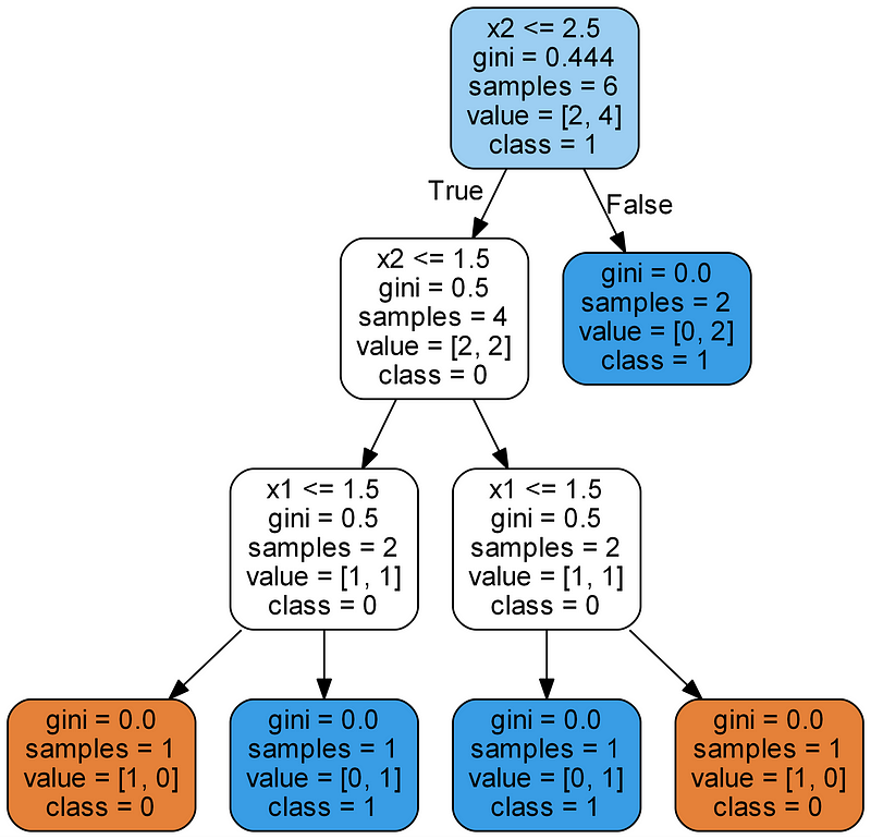
All the nodes, except the leaf nodes (colored terminal nodes), have 5 parts:
- Question asked about the data based on a value of a feature. Each question has either a True or False answer that splits the node. Based on the answer to the question, a data point moves down the tree.
gini: The Gini Impurity of the node. The average weighted Gini Impurity decreases as we move down the tree.samples: The number of observations in the node.value: The number of samples in each class. For example, the top node has 2 samples in class 0 and 4 samples in class 1.class: The majority classification for points in the node. In the case of leaf nodes, this is the prediction for all samples in the node.
The leaf nodes do not have a question because these are where the final
predictions are made. To classify a new point, simply move down the tree, using
the features of the point to answer the questions until you arrive at a leaf
node where the class is the prediction.
To make see the tree in a different way, we can draw the splits built by the decision tree on the original data.
 Splits made by the decision tree.
Each split is a single line that divides data points into nodes based on feature values. For this simple problem and with no limit on the maximum depth, the divisions place each point in a node with only points of the same class. (Again, later we’ll see that this perfect division of the training *data might not be what we want because it can lead to *overfitting.)
Gini Impurity
At this point it’ll be helpful to dive into the concept of Gini Impurity (the math is not intimidating!) The Gini Impurity of a node is the probability that a randomly chosen sample in a node would be incorrectly labeled if it was labeled by the distribution of samples in the node. For example, in the top (root) node, there is a 44.4% chance of incorrectly classifying a data point chosen at random based on the sample labels in the node. We arrive at this value using the following equation:
 Gini impurity of a node n.
The Gini Impurity of a node n is 1 minus the sum over all the classes J (for
a binary classification task this is 2) of the fraction of examples in each
class p_i squared. That might be a little confusing in words, so let’s work
out the Gini impurity of the root node.
 Gini Impurity of the root node
At each node, the decision tree searches through the features for the value to split on that results in the greatest reduction in Gini Impurity. (An alternative for splitting nodes is using the information gain, a related concept).
It then repeats this splitting process in a greedy, recursive procedure until it reaches a maximum depth, or each node contains only samples from one class. The weighted total Gini Impurity at each level of tree must decrease. At the second level of thetree, the total weighted Gini Impurity is 0.333:
 Total Weighted Gini Impurity of Tree Second Level
(The Gini Impurity of each node is weighted by the fraction of points from the parent node in that node.) You can continue to work out the Gini Impurity for each node (check the visual for the answers). Out of some basic math, a powerful model emerges!
Eventually, the weighted total Gini Impurity of the last layer goes to 0 meaning each node is completely pure and there is no chance that a point randomly selected from that node would be misclassified. While this may seem like a positive, it means that the model may potentially be overfitting because the nodes are constructed only using training data.
Overfitting: Or Why a Forest is better than One Tree
You might be tempted to ask why not just use one decision tree? It seems like the perfect classifier since it did not make any mistakes! A critical point to remember is that the tree made no mistakes on the training data. We expect this to be the case since we gave the tree the answers and didn’t limit the max depth (number of levels). The objective of a machine learning model is to generalize well to new data it has never seen before.
Overfitting occurs when we have a very flexible model (the model has a high capacity) which essentially memorizes the training data by fitting it closely. The problem is that the model learns not only the actual relationships in the training data, but also any noise that is present. A flexible model is said to have high variance because the learned parameters (such as the structure of the decision tree) will vary considerably with the training data.
On the other hand, an inflexible model is said to have high bias because it makes assumptions about the training data (it’s biased towards pre-conceived ideas of the data.) For example, a linear classifier makes the assumption that the data is linear and does not have the flexibility to fit non-linear relationships. An inflexible model may not have the capacity to fit even the training data and in both cases — high variance and high bias — the model is not able to generalize well to new data.
The balance between creating a model that is so flexible it memorizes the training data versus an inflexible model that can’t learn the training data is known as the bias-variance tradeoff and is a foundational concept in machine learning.
The reason the decision tree is prone to overfitting when we don’t limit the maximum depth is because it has unlimited flexibility, meaning that it can keep growing until it has exactly one leaf node for every single observation, perfectly classifying all of them. If you go back to the image of the decision tree and limit the maximum depth to 2 (making only a single split), the classifications are no longer 100% correct. We have reduced the variance of the decision tree but at the cost of increasing the bias.
As an alternative to limiting the depth of the tree, which reduces variance (good) and increases bias (bad), we can combine many decision trees into a single ensemble model known as the random forest.
Random Forest
The random forest is a model made up of many decision trees. Rather than just simply averaging the prediction of trees (which we could call a “forest”), this model uses two key concepts that gives it the name random:
- Random sampling of training data points when building trees
- Random subsets of features considered when splitting nodes
Random sampling of training observations
When training, each tree in a random forest learns from a random sample of the data points. The samples are drawn with replacement, known as bootstrapping, which means that some samples will be used multiple times in a single tree. The idea is that by training each tree on different samples, although each tree might have high variance with respect to a particular set of the training data, overall, the entire forest will have lower variance but not at the cost of increasing the bias.
At test time, predictions are made by averaging the predictions of each decision tree. This procedure of training each individual learner on different bootstrapped subsets of the data and then averaging the predictions is known as bagging, short for bootstrap aggregating.
Random Subsets of features for splitting nodes
The other main concept in the random forest is that only a subset of all the
features are considered for splitting each
node
in each decision tree. Generally this is set to sqrt(n_features) for
classification meaning that if there are 16 features, at each node in each tree,
only 4 random features will be considered for splitting the node. (The random
forest can also be trained considering all the features at every node as is
common in regression. These options can be controlled in the Scikit-Learn
Random Forest
implementation).
If you can comprehend a single decision tree, the idea of bagging, and random subsets of features, then you have a pretty good understanding of how a random forest works:
The random forest combines hundreds or thousands of decision trees, trains each one on a slightly different set of the observations, splitting nodes in each tree considering a limited number of the features. The final predictions of the random forest are made by averaging the predictions of each individual tree.
To understand why a random forest is better than a single decision tree imagine the following scenario: you have to decide whether Tesla stock will go up and you have access to a dozen analysts who have no prior knowledge about the company. Each analyst has low bias because they don’t come in with any assumptions, and is allowed to learn from a dataset of news reports.
This might seem like an ideal situation, but the problem is that the reports are likely to contain noise in addition to real signals. Because the analysts are basing their predictions entirely on the data — they have high flexibility — they can be swayed by irrelevant information. The analysts might come up with differing predictions from the same dataset. Moreover, each individual analyst has high variance and would come up with drastically different predictions if given a different training set of reports.
The solution is to not rely on any one individual, but pool the votes of each analyst. Furthermore, like in a random forest, allow each analyst access to only a section of the reports and hope the effects of the noisy information will be cancelled out by the sampling. In real life, we rely on multiple sources (never trust a solitary Amazon review), and therefore, not only is a decision tree intuitive, but so is the idea of combining them in a random forest.
Random Forest in Practice
Next, we’ll build a random forest in Python using Scikit-Learn. Instead of learning a simple problem, we’ll use a real-world dataset split into a training and testing set. We use a test set as an estimate of how the model will perform on new data which also lets us determine how much the model is overfitting.
Dataset
The problem we’ll solve is a binary classification task with the goal of
predicting an individual’s health. The features are socioeconomic and lifestyle
characteristics of individuals and the label is 0 for poor health and 1 for
good health. This dataset was collected by the Centers for Disease Control and
Prevention and is available
here.
 Sample of Data
Generally, 80% of a data science project is spent cleaning, exploring, and making features out of the data. However, for this article, we’ll stick to the modeling. (For details of the other steps, look at this article).
This is an imbalanced classification problem, so accuracy is not an appropriate metric. Instead we’ll measure the Receiver Operating Characteristic Area Under the Curve (ROC AUC), a measure from 0 (worst) to 1 (best) with a random guess scoring 0.5. We can also plot the ROC curve to assess a model.
The notebook contains the implementation for both the decision tree and the random forest, but here we’ll just focus on the random forest. After reading in the data, we can instantiate and train a random forest as follows:
After a few minutes to train, the model is ready to make predictions on the testing data as follows:
We make class predictions (predict) as well as predicted probabilities
(predict_proba) to calculate the ROC AUC. Once we have the testing
predictions, we can calculate the ROC AUC.
Results
The final testing ROC AUC for the random forest was 0.87 compared to 0.67 for the single decision tree with an unlimited max depth. If we look at the training scores, both models achieved 1.0 ROC AUC, which again is as expected because we gave these models the training answers and did not limit the maximum depth of each tree.
Although the random forest overfits (doing better on the training data than on the testing data), it is able to generalize much better to the testing data than the single decision tree. The random forest has lower variance (good) while maintaining the same low bias (also good) of a decision tree.
We can also plot the ROC curve for the single decision tree (top) and the random forest (bottom). A curve to the top and left is a better model:
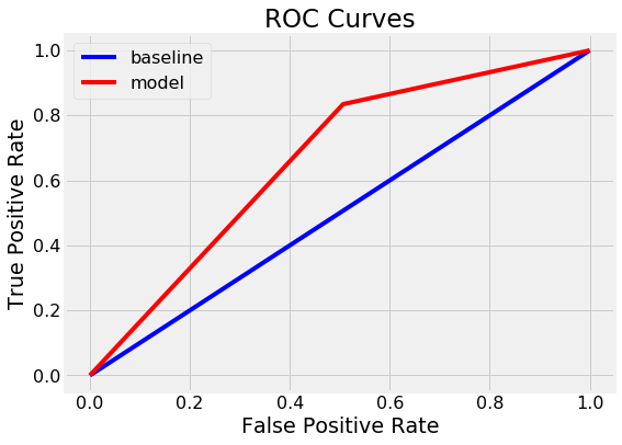
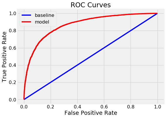
The random forest significantly outperforms the single decision tree.
Another diagnostic measure of the model we can take is to plot the confusion matrix for the testing predictions (see the notebook for details):
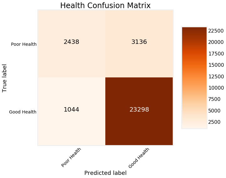
This shows the predictions the model got correct in the top left and bottom right corners and the predictions missed by the model in the lower left and upper right. We can use plots such as these to diagnose our model and decide whether it’s doing well enough to put into production.
Feature Importances
The feature importances in a random forest indicate the sum of the reduction in Gini Impurity over all the nodes that are split on that feature. We can use these to try and figure out what predictor variables the random forest considers most important. The feature importances can be extracted from a trained random forest and put into a Pandas dataframe as follows:
Feature importances can give us insight into a problem by telling us what
variables are the most discerning between classes. For example, here DIFFWALK,
indicating whether the patient has difficulty walking, is the most important
feature which makes sense in the problem context.
Feature importances can be used for feature engineering by building additional features from the most important. We can also use feature importances for feature selection by removing low importance features.
Visualize Tree in Forest
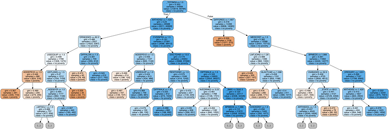
Finally, we can visualize a single decision tree in the forest. This time, we have to limit the depth of the tree otherwise it will be too large to be converted into an image. To make the figure below, I limited the maximum depth to 6. This still results in a large tree that we can’t completely parse! However, given our deep dive into the decision tree, we grasp how our model is working.
Next Steps
A further step is to optimize the random forest which we can do through random
search using the RandomizedSearchCV in
Scikit-Learn.
Optimization refers to finding the best hyperparameters for a model on a given
dataset. The best hyperparameters will vary between datasets, so we have to
perform optimization (also called model tuning) separately on each datasets.
I like to think of model tuning as finding the best settings for a machine learning algorithm. Examples of what we might optimize in a random forest are the number of decision trees, the maximum depth of each decision tree, the maximum number of features considered for splitting each node, and the maximum number of data points required in a leaf node.
For an implementation of random search for model optimization of the random forest, refer to the Jupyter Notebook.
Complete Running Example
The below code is created with repl.it and presents a complete interactive running example of the random forest in Python. Feel free to run and change the code (loading the packages might take a few moments).
Complete Python example of random forest.
Conclusions
While we can build powerful machine learning models in Python without understanding anything about them, I find it’s more effective to have knowledge about what is occurring behind the scenes. In this article, we not only built and used a random forest in Python, but we also developed an understanding of the model by starting with the basics.
We first looked at an individual decision tree, the building block of a random forest, and then saw how we can overcome the high variance of a single decision tree by combining hundreds of them in an ensemble model known as a random forest. The random forest uses the concepts of random sampling of observations, random sampling of features, and averaging predictions.
The key concepts to understand from this article are:
- Decision tree: an intuitive model that makes decisions based on a sequence of questions asked about feature values. Has low bias and high variance leading to overfitting the training data.
- Gini Impurity: a measure that the decision tree tries to minimize when splitting each node. Represents the probability that a randomly selected sample from a node will be incorrectly classified according to the distribution of samples in the node.
- Bootstrapping: sampling random sets of observations with replacement.
- Random subsets of features: selecting a random set of the features when considering splits for each node in a decision tree.
- Random Forest: ensemble model made of many decision trees using bootstrapping, random subsets of features, and average voting to make predictions. This is an example of a bagging ensemble.
- Bias-variance tradeoff: a core issue in machine learning describing the balance between a model with high flexibility (high variance) that learns the training data very well at the cost of not being able to generalize to new data , and an inflexible model (high bias) that cannot learn the training data. A random forest reduces the variance of a single decision tree leading to better predictions on new data.
Hopefully this article has given you the confidence and understanding needed to start using the random forest on your projects. The random forest is a powerful machine learning model, but that should not prevent us from knowing how it works. The more we know about a model, the better equipped we will be to use it effectively and explain how it makes predictions.
As always, I welcome comments, feedback, and constructive criticism. I can be reached on Twitter @koehrsen_will. This article was originally published on enlight, an open-source community for studying machine learning. I would like to thank enlight and also repl.it for hosting the code in the article.