
Deep Neural Network Classifier
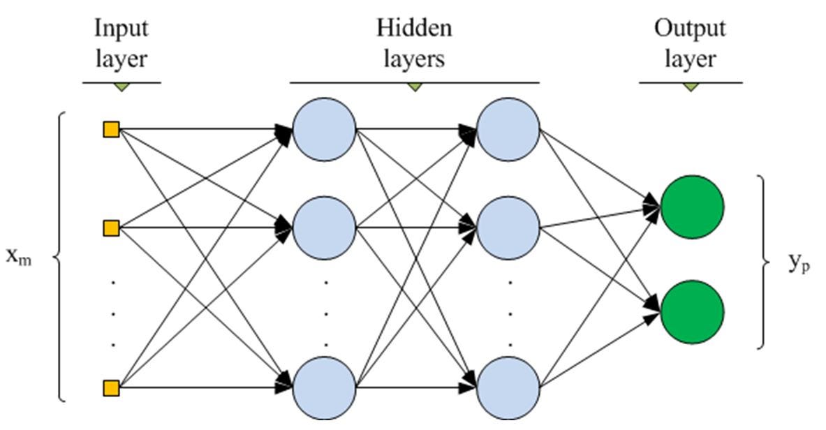
A Scikit-learn compatible Deep Neural Network built with TensorFlow
TensorFlow is a open-source deep learning library with tools for building almost any type of neural network (NN) architecture. Originally developed by the Google Brain team, TensorFlow has democratized deep learning by making it possible for anyone with a personal computer to build their own deep NN, convolutional NN, recurrent NN, that can be applied in a diverse array of fields. Scikit-learn is an open-source machine learning library with implementations for developing and perfecting numerous types of machine learning models. Both libraries feature high-level functionality that make designing models in Python relatively simple, but both libraries also have their limitations: Scikit-learn has no native implementation for neural networks, while Tensorflow has no built-in functionality to efficiently evaluate a wide range of network hyperparameters. We can overcome both these problems by developing a Scikit-learn compatible deep neural network class using TensorFlow. We can then take advantage of Scikit-learn built-in model hyperparameter tuning tools such as GridSearchCV or RandomizedSearchCV to optimize our deep neural network.
All the code is written in Python and available on GitHub on my machine learning projects repository. The main files are dnn_classifier.py, the Python file containing the classifier, and Deep Neural Network Classifier.ipynb, a Jupyter Notebook with the implementations of the neural network. I welcome any criticism/comments and the code will change as I improve it over time. This project was inspired and aided by Hands-On Machine Learning with Scikit-Learn and TensorFlow by Aurelien Geron.
Code
Here is the code for the deep neural network class in its entirety.
import numpy as np
import tensorflow as tf
from sklearn.base import BaseEstimator, ClassifierMixin
from sklearn.exceptions import NotFittedError
from datetime import datetime

# He et al. initialization from [https://arxiv.org/abs/1502.01852](https://arxiv.org/abs/1502.01852?)
he_init = tf.contrib.layers.variance_scaling_initializer()

# This class inherits from Sklearn's BaseEstimator and ClassifierMixin
class DNNClassifier(BaseEstimator, ClassifierMixin):
 def __init__(self, n_hidden_layers=4, n_neurons=50,           optimizer_class=tf.train.AdamOptimizer, learning_rate=0.01,   batch_size=20, activation=tf.nn.elu, initializer=he_init,    batch_norm_momentum=None, dropout_rate=None,       max_checks_without_progress=20,show_progress=10,      tensorboard_logdir=None, random_state=None):

  # Initialize the class with sensible default hyperparameters
  self.n_hidden_layers = n_hidden_layers
  self.n_neurons = n_neurons
  self.optimizer_class = optimizer_class
  self.learning_rate = learning_rate
  self.batch_size = batch_size
  self.activation = activation
  self.initializer = initializer
  self.batch_norm_momentum = batch_norm_momentum
  self.dropout_rate = dropout_rate
  self.max_checks_without_progress = max_checks_without_progress
  self.show_progress = show_progress
  self.random_state = random_state
  self.tensorboard_logdir = tensorboard_logdir
  self._session = None #Instance variables preceded by _ are private members

 def _dnn(self, inputs):
  '''This method builds the hidden layers and
   Provides for implementation of batch normalization and dropout'''

for layer in range(self.n_hidden_layers):

# Apply dropout if specified
   if self.dropout_rate:
    inputs = tf.layers.dropout(inputs, rate=self.dropout_rate,        training=self._training)
   # Create the hidden layer
   inputs = tf.layers.dense(inputs, self.n_neurons,
          activation=self.activation,
          kernel_initializer=self.initializer,
          name = "hidden{}".format(layer+1))

# Apply batch normalization if specified
   if self.batch_norm_momentum:
    inputs = tf.layers.batch_normalization(inputs,momentum=          self.batch_norm_momentum,
             training=self._training)

   # Apply activation function
   inputs = self.activation(inputs, name="hidden{}_out".format(layer+1))
  return inputs

 def _construct_graph(self, n_inputs, n_outputs):
  '''This method builds the complete Tensorflow computation graph
   n_inputs: number of features
   n_outputs: number of classes
  '''

if self.random_state:
   tf.set_random_seed(self.random_state)
   np.random.seed(self.random_state)

  # Placeholders for training data, labels are class exclusive integers
  X = tf.placeholder(tf.float32, shape=[None, n_inputs], name="X")
  y = tf.placeholder(tf.int32, shape=[None], name="y")

  # Create a training placeholder
  if self.batch_norm_momentum or self.dropout_rate:
   self._training = tf.placeholder_with_default(False, shape=[], name="training")
  else:
   self._training = None

  # Output after hidden layers
  pre_output = self._dnn(X)

  # Outputs from output layer
  logits = tf.layers.dense(pre_output, n_outputs, kernel_initializer=he_init, name="logits")
  probabilities = tf.nn.softmax(logits, name="probabilities")

  ''' Cost function is cross entropy and loss is average cross entropy. Sparse softmax must be used because shape of logits is [None, n_classes] and shape of labels is [None]'''
  xentropy = tf.nn.sparse_softmax_cross_entropy_with_logits(labels=y,               logits=logits)
  loss = tf.reduce_mean(xentropy, name="loss")

  '''Optimizer and training operation. The control dependency is necessary for implementing batch normalization. The training operation must be dependent on the batch normalization.'''

optimizer = self.optimizer_class(learning_rate=self.learning_rate)
  update_ops = tf.get_collection(tf.GraphKeys.UPDATE_OPS)
  with tf.control_dependencies(update_ops):
   training_op = optimizer.minimize(loss)

  # Metrics for evaluation
  correct = tf.nn.in_top_k(logits, y, 1)
  accuracy = tf.reduce_mean(tf.cast(correct, tf.float32),name="accuracy")

# Initializer and saver
  init = tf.global_variables_initializer()
  saver = tf.train.Saver()

  if self.tensorboard_logdir:
   now = datetime.utcnow().strftime('%Y%m%d-%H%M%S')
   tb_logdir = self.tensorboard_logdir + "/run-{}".format(now)
   cost_summary = tf.summary.scalar("validation_loss", loss)
   acc_summary = tf.summary.scalar("validation_accuracy", accuracy)
   merged_summary = tf.summary.merge_all()
   file_writer = tf.summary.FileWriter(tb_logdir,              tf.get_default_graph())

   self._merged_summary = merged_summary
   self._file_writer = file_writer

  self._X, self._y = X, y
  self._logits = logits
  self._probabilities = probabilities
  self._loss = loss
  self._training_op = training_op
  self._accuracy = accuracy
  self._init, self._saver = init, saver

 def close_session(self):
  if self._session:
   self._session.close()

 def _get_model_parameters(self):
  # Retrieves the value of all the variables in the network
  with self._graph.as_default():
   gvars = tf.get_collection(tf.GraphKeys.GLOBAL_VARIABLES)
  return {gvar.op.name: value for gvar, value in
    zip(gvars, self._session.run(gvars))}

 def _restore_model_parameters(self, model_params):
  # Restores the value of all variables using tf assign operations
  # First retrieve the list of all the graph variables
  gvar_names = list(model_params.keys())

  # Then retrieve all the assignment operations in the graph
  assign_ops = {gvar_name: self._graph.get_operation_by_name(gvar_name +     "/Assign") for gvar_name in gvar_names}

# Fetch the initialization values of the assignment operations
  '''graph.get_operation_by_name(operation).inputs returns the input to the given operation; because these are all assignment operations, the second argument to inputs is the value assigned to the variable'''
  init_values = {gvar_name: assign_op.inputs[1] for gvar_name, assign_op      in assign_ops.items()}
  # Create a dictionary mapping initial values to values after training
  feed_dict = {init_values[gvar_name]: model_params[gvar_name] for gvar_name in gvar_names}
  # Assign the trained value to all the variables in the graph
  self._session.run(assign_ops, feed_dict=feed_dict)

 def fit(self, X, y, n_epochs=100, X_valid=None, y_valid=None):
  # Method to train the model. Implements early stopping if validation data is provided

  self.close_session()
  n_inputs = X.shape[1] # Number of features

  # If labels are provided in one_hot form, convert to integer class labels
  y = np.array(y)
  y_valid = np.array(y_valid)

  if len(y.shape) == 2:
   y = np.argmax(y, axis=1)

  if len(y_valid.shape) == 2:
   y_valid = np.argmax(y_valid, axis=1)

self.classes_ = np.unique(y)
  n_outputs = len(self.classes_) # Number of classes

  # Tensorflow expects labels from 0 to n_classes - 1\.
  self.class_to_index_ = {label: index for index, label in enumerate(self.classes_)}
  labels = [self.class_to_index_[label] for label in y]
  y = np.array(labels, dtype=np.int32)

  self._graph = tf.Graph()

  # Build the computation graph with self as default graph
  with self._graph.as_default():
   self._construct_graph(n_inputs, n_outputs)

  # Early stopping parameters
  checks_without_progress = 0
  best_loss = np.float("inf")
  best_parameters = None

  self._session = tf.Session(graph=self._graph)

with self._session.as_default() as sess:
   # Initialize all variables
   self._init.run()
   num_instances = X.shape[0] # Total number of training instances
   for epoch in range(n_epochs):
    rnd_idx = np.random.permutation(num_instances)
    for rnd_indices in np.array_split(rnd_idx, num_instances // self.batch_size):
     X_batch, y_batch = X[rnd_indices], y[rnd_indices]
     feed_dict = {self._X: X_batch, self._y: y_batch}
     if self._training is not None:
      feed_dict[self._training] = True
     train_acc, _ = sess.run([self._accuracy,self._training_op],      feed_dict)

# Early stopping implementation
    if X_valid is not None and y_valid is not None:
     feed_dict_valid = {self._X: X_valid, self._y: y_valid}

# Write summary for tensorboard
     if self.tensorboard_logdir:
      val_acc, val_loss, summary = sess.run([self._accuracy, self._loss, self._merged_summary], feed_dict=feed_dict_valid)

self._file_writer.add_summary(summary, epoch)

else:
      val_acc, val_loss = sess.run([self._accuracy, self._loss], feed_dict=feed_dict_valid)

     # Show training progress every show_progress epochs
     if self.show_progress:
      if epoch % self.show_progress == 0:
       print("Epoch: {} Current training accuracy: {:.4f} Validation Accuracy: {:.4f} Validation Loss {:.6f}".format(
        epoch+1, train_acc, val_acc, val_loss))

# Check to see if model is improving
     if val_loss < best_loss:
      best_loss = val_loss
      checks_without_progress = 0
      best_parameters = self._get_model_parameters()
     else:
      checks_without_progress += 1

if checks_without_progress > self.max_checks_without_progress:
      print("Stopping Early! Loss has not improved in {} epochs".format(
             self.max_checks_without_progress))
      break

    # No validation set provided
    else:
     if self.show_progress:
      if epoch % self.show_progress == 0:
       print("Epoch: {} Current training accuracy: {:.4f}".format(
        epoch+1, train_acc))

   # In the case of early stopping, restore the best weight values
   if best_parameters:
    self._restore_model_parameters(best_parameters)
    return self

 def predict_probabilities(self, X):
  # Predict the probabilities of each class
  if not self._session:
   raise NotFittedError("This %s instance is not fitted yet" % self.__class__.__name__)
  with self._session.as_default() as sess:
   return self._probabilities.eval(feed_dict={self._X: X})

def predict(self, X):
  # Predict the classes themselves and return with shape=(None,)
  class_indices = np.argmax(self.predict_probabilities(X), axis=1)
  predictions = np.array([[self.classes_[class_index]] for class_index in class_indices], dtype=np.int32)
  return np.reshape(predictions, (-1,))

 def save(self, path):
  # Save the model to provided path
  self._saver.save(self._session, path)
Using the Model with the MNIST dataset
Now that we have developed the model, it’s time to put it to use on some traditional machine learning datasets. To test it out, we can use the MNIST hand-written digit dataset, a collection of numbers written out by hand and labeled.
First we can import the classifier object and load the MNIST data.
from dnn_classifier import DNNClassifier
from tensorflow.examples.tutorials.mnist import input_data

mnist = input_data.read_data_sets("/tmp/data")

X_train = mnist.train.images
y_train = mnist.train.labels

X_valid = mnist.validation.images
y_valid = mnist.validation.labels

X_test = mnist.test.images
y_test = mnist.test.labels
Then we can instantiate an instance of the class using the default hyperparameters (we’ll pass in a log directory so we can track training on TensorBoard and a random state to ensure consistent output across runs).
dnn = DNNClassifier(tensorboard_logdir="/tensorboard_stats", random_state=42)
Then we can train the classifier and pass in a validation set to see progress. The classifier prints the statistics every show_progress epochs (which was left at the default 10). Because we used a validation set, the classifier will implement early stopping when training. This means that if the validation loss does not improve for a given number of epochs, the classifier will stop training because further iterations will likely not improve performance. Each iteration that the validation loss does decrease, the model weights are saved so that the best model can be restored at the end of training. This is one way to combat overfitting on the training set and creating a classifier with a lower variance that can better generalize to novel data.
dnn.fit(X_train, y_train, 100, X_valid, y_valid)

Output:
Epoch: 1 Current training accuracy: 0.9500 Validation Accuracy: 0.9408 Validation Loss 0.226019
Epoch: 11 Current training accuracy: 1.0000 Validation Accuracy: 0.9538 Validation Loss 0.214198
Epoch: 21 Current training accuracy: 1.0000 Validation Accuracy: 0.9390 Validation Loss 0.313651
Stopping Early! Loss has not improved in 20 epochs
We can also launch Tensorboard from Windows PowerShell to observe the training curves:
tensorboard --logdir=tensorboard/stats
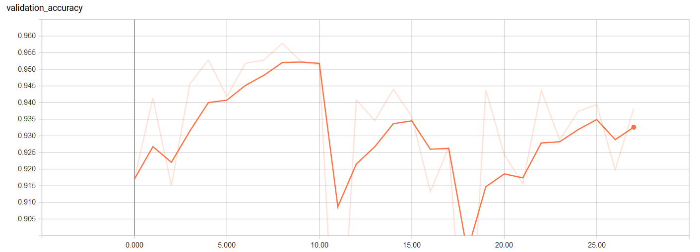 Validation Accuracy
We can see that the validation accuracy peaked at epoch 10. This is valuable information because it shows that we might only need to train for 1/10th of the original amount of training epochs. The validation accuracy also begins to increase towards the end (before it is stopped early) suggesting that we might benefit from a few more training epochs.
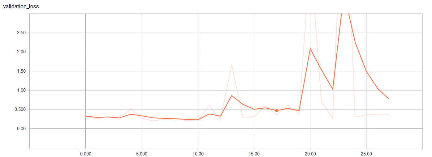 Validation Loss
It looks like the minimum validation loss occurred near the first iteration and then rose after that before heading back down. Perhaps it we increase the maximum number of epochs without a decrease in the validation loss, we can achieve better accuracy. The final accuracy on the test set can be assessed:
from sklearn.metrics import accuracy_score

y_pred = dnn.predict(X_test)
print("Accuracy on the test set: {:.2f}%".format(accuracy_score(y_test, y_pred) * 100))

Output:
Accuracy on the test set: 94.76%
Our default neural network achieves near 95% accuracy on identifying hand-written digits. That’s not great, but we have not optimized any of the network hyperparameters. Let’s take a look at a couple of predictions by plotting the handwritten images themselves and the probability (confidence) that the classifier has for each digit:
import matplotlib.pyplot as plt
import numpy as np

# For plotting within the Jupyter Notebook
%matplotlib inline

# Pick random examples to predict
example_indices = np.random.randint(len(X_test), size=4)

# Plot the image itself and the predicted class probabilities
for i, image_index in enumerate(example_indices):
    probabilities = dnn.predict_probabilities(X_test[image_index].reshape(-1, 784))
    plt.figure(figsize=(8,8))
    plt.imshow(X_test[image_index].reshape(28,28), cmap="binary")
    plt.show()
    for label, probability in zip(dnn.classes_, probabilities[0]):
        print("{} Confidence: {:.2f}%".format(label, probability*100))
And the results
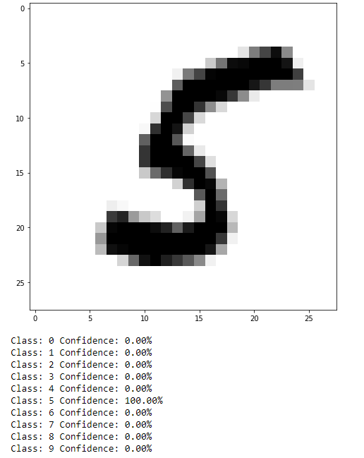
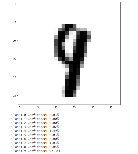
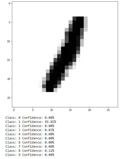
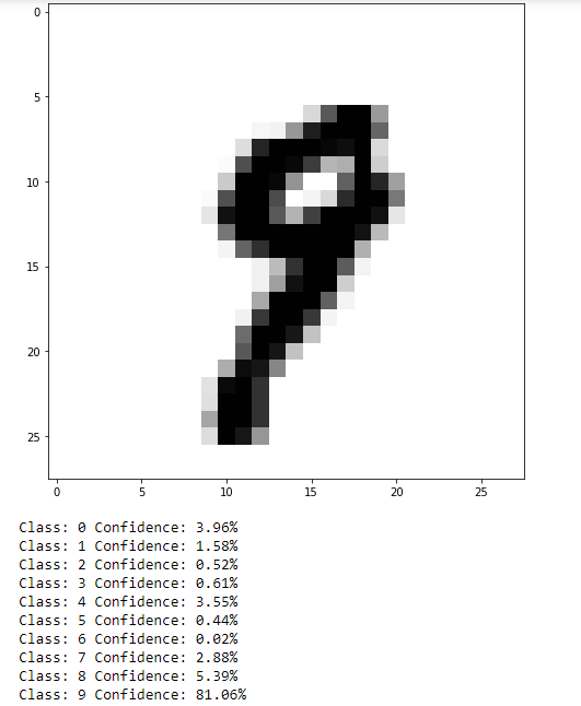 As can be seen, not too bad. This isn’t a very difficult task, but it can be easy to see how results such as this translated to more practical data, such as self-driving cars identifying objects in their environment (although that is likely a task better suited to convolutional NN or a CNN in combination with a recurrent NN).
Scikit-learn Hyperparameter Tuning
We can significantly improve the accuracy by tuning the hyperparameters of the model using Randomized Search CV and/or Grid Search CV. This is the reason why we made the model compatible with Scikit-learn in the first place. We will create a sensible set of parameter distributions and let Scikit-learn evaluate a range of them for us. This process may take several hours to days depending on your set-up. I would recommend running this on your GPU if possible or investing in setting up a Google Cloud compute instance (they will give you $300 in credit when you create a new account).
from sklearn.model_selection import RandomizedSearchCV

import tensorflow as tf

# We do not need to print out progress for every classifier
dnn = DNNClassifier(show_progress=None, random_state=42)

# Hyperparameters of the neural network to test
parameter_distributions = {
    'n_hidden_layers': [3, 4, 5],
    'n_neurons': [40, 50, 100],
    'batch_size': [64, 128],
    'learning_rate':[0.01, 0.005],
    'activation': [tf.nn.elu, tf.nn.relu],
    'max_checks_without_progress': [20, 30],
    'batch_norm_momentum': [None, 0.9],
    'dropout_rate': [None, 0.5]
}

# Adjust iterations to a number sensible for your set-up
random_search = RandomizedSearchCV(dnn, parameter_distributions, n_iter=50, scoring='accuracy', verbose=2)

# Train the model
random_search.fit(X_train, y_train)
Let’s see what the best hyperparameter configuration is from the random search:
random_search.best_params_

Output:
{'activation': <function tensorflow.python.ops.gen_nn_ops.elu>,
 'batch_norm_momentum': 0.9,
 'batch_size': 64,
 'dropout_rate': None,
 'learning_rate': 0.005,
 'max_checks_without_progress': 20,
 'n_hidden_layers': 3,
 'n_neurons': 100}
And the performance on the test set:
best_mnist_dnn = random_search.best_estimator_
mnist_predictions = best_mnist_dnn.predict(X_test)

print("Accuracy on test set: {:.2f}%".format(accuracy_score(y_test, mnist_predictions) * 100))

Output:

Accuracy on test set: 98.18%
Not too bad after a relatively small search through the hyperparameter space. We only used 15 different combinations, so it is likely that a better tuned network exists. After we use a randomized search, we can further improve our model by doing a grid search focused around the best settings returned by the search.
dnn = DNNClassifier(show_progress=None, random_state=42)

parameter_grid = {
    'n_hidden_layers': [3],
    'n_neurons': [75, 100, 125, 150],
    'batch_size': [64],
    'learning_rate':[0.005],
    'activation': [tf.nn.elu],
    'max_checks_without_progress': [20, 25],
    'batch_norm_momentum': [0.9, 0.95],
}

grid_search = GridSearchCV(dnn, parameter_grid, scoring='accuracy', verbose=2)
grid_search.fit(X_train, y_train)

predictions = grid_search.best_estimator_.predict(X_test)
accuracy_score(predictions, y_test)

Output:
Score on test set: 98.21%
Still not perfect, but improving. The best model likely exists out there but we haven’t found it yet. For now, we’ll take 98.2% accuracy which is probably better than I would be able to do (I know that when I write numbers, people can usually identify them 80% of the time).
As a final step, we want to save our best model weights.
grid_search.best_estimator_.save("models/mnist_grid_best")
This will save all of the model weights so if we create an identical TensorFlow graph, we can put all of these weights into the graph and there will be no need for the time-consuming training step (assuming we still want to classify hand-written digits. If we change the task, we will have to re-train the model).
Titanic Dataset
Let’s take a brief look at the performance on another standard machine learning dataset, the Titanic passenger list. The goal with this dataset is to predict which passengers survived and which did not based on age, passenger class, gender, fare paid, cabin, destination, etc. This is a historically accurate dataset and quite interesting to investigate.
We can first load in the dataset into a Pandas dataframe and look at the info:
import pandas as pd
import numpy as np

titanic = pd.read_excel("datasets/titanic.xls")
titanic.head(10)
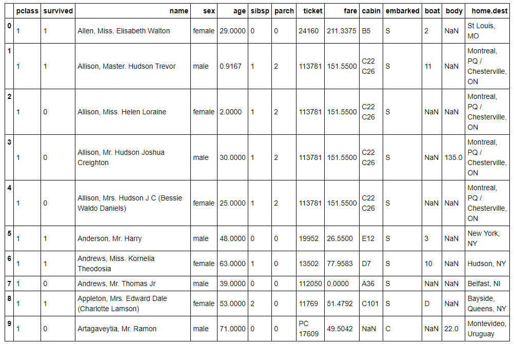 Example of Titanic Data
The labels will be whether or not the passenger survived (1 for yes and 0 for no). The features will be all the columns except for survived (that would make things a little too easy), name, body identification number, and boat.
Let’s get the data into training and testing sets:
# Labels are survived, features need to drop survived, body, name
titanic_labels = np.array(titanic['survived'])
titanic_features = titanic.drop(['survived', 'name', 'body', 'boat'], axis=1)

# One-hot encode the categorical variables
titanic_features = pd.get_dummies(titanic_features)

#Set NAN to 0
titanic_features = np.nan_to_num(titanic_features)
titanic_features = np.array(titanic_features)

from sklearn.model_selection import train_test_split

# Put one quarter of data into testing set
X_train, X_test, y_train, y_test = train_test_split(titanic_features, titanic_labels, test_size=0.25)

print(X_train.shapedd, X_test.shape)

Output:
(983, 2813) (328, 2813)
It looks like we have 981 passengers in our training data and 328 in our testing data. After one-hot encoding, there are 2831 features to use to determine whether or no a passenger survived. We can now train on the data:
dnn = DNNClassifier(show_progress=10, random_state=42)

dnn.fit(X_train, y_train, n_epochs=100)

Output:
Epoch: 1 Current training accuracy: 0.8000
Epoch: 11 Current training accuracy: 1.0000
Epoch: 21 Current training accuracy: 1.0000
Epoch: 31 Current training accuracy: 1.0000
Epoch: 41 Current training accuracy: 1.0000
Epoch: 51 Current training accuracy: 1.0000
Epoch: 61 Current training accuracy: 1.0000
Epoch: 71 Current training accuracy: 1.0000
Epoch: 81 Current training accuracy: 1.0000
Epoch: 91 Current training accuracy: 1.0000
Well, we are clearly overfitting the training data! We can reduce that by implementing dropout, reducing the number of hidden layers, reducing the number of neurons per layer, or implementing early stopping. For now let’s check out the accuracy on the test set and then implement dropout:
from sklearn.metrics import accuracy_score

survival_predictions= dnn.predict(X_test)
print("Score on test set: {:.2f}%".format(accuracy_score(y_test, survival_predictions) * 100))

Output:
Score on test set: 75.91%
Even though we are badly overfitting the training data, our classifier can still pick with 76% accuracy whether or not a passenger on the Titanic would survive the journey. Let’s try dropout with 0.75 of the input to each layer retained:
dnn = DNNClassifier(dropout_rate=0.25, show_progress=10, random_state=42)
dnn.fit(X_train, y_train, n_epochs=100)

survival_predictions= dnn.predict(X_test)
print("Score on test set: {:.2f}%".format(accuracy_score(y_test, survival_predictions) * 100))

Output:

Epoch: 1 Current training accuracy: 0.5000
Epoch: 11 Current training accuracy: 0.8500
Epoch: 21 Current training accuracy: 0.8500
Epoch: 31 Current training accuracy: 0.8500
Epoch: 41 Current training accuracy: 0.9000
Epoch: 51 Current training accuracy: 0.9000
Epoch: 61 Current training accuracy: 0.9500
Epoch: 71 Current training accuracy: 0.9500
Epoch: 81 Current training accuracy: 0.9000
Epoch: 91 Current training accuracy: 0.8500
Score on test set: 76.83%
Well, dropout clearly reduced the extent of overfitting as evidenced by the lower scores on the test set. However, it did not substantially improve overall accuracy on the test set (dropout of 0.5 achieved 75% accuracy). We could use randomized search to narrow down the range of hyperparameters and then grid search to optimize the network but I’ll leave that for now.
Just for fun, let’s put myself and my dad on the Titanic and see what our survival chances are. I will put in some true information (I’ll be generous with my dad’s age) and then randomly choose other feature values.
import random

# Randomly choose cabin, ticket, destination, and boat
my_cabin = random.choice(titanic['cabin'])
father_cabin = random.choice(titanic['cabin'])
my_ticket = random.choice(titanic['ticket'])
father_ticket = random.choice(titanic['ticket'])
my_dest = random.choice(titanic['home.dest'])
father_dest = random.choice(titanic['home.dest'])

me = [2, 1, "Koehrsen, William", "male", 21, 2, 2, my_ticket, 50, my_cabin, 'S', my_boat, np.nan, my_dest]
father = [1, 1, "Koehrsen, Craig", "male", 50, 2, 2, father_ticket, 200, father_cabin, 'S', father_boat, np.nan, father_dest]

titanic.loc[1309] = me
titanic.loc[1310] = father

titanic_with_family = titanic.drop(['survived','body'], axis=1)
titanic_with_family = pd.get_dummies(titanic_with_family)
titanic_with_family = np.nan_to_num(titanic_with_family)

me = titanic_with_family[1309]
father = titanic_with_family[1310]
my_survival_chances = dnn.predict_probabilities(me.reshape(-1, X_train.shape[1]))
father_survival_chances = dnn.predict_probabilities(father.reshape(-1, X_train.shape[1]))

print('My survival chances: {0[0]} = {1[0][0]:.6f}%, {0[1]} = {1[0][1]:.6f}%'.format(dnn.classes_, my_survival_chances*100))
print('Father\'s survival chances: {0[0]} = {1[0][0]:.6f}%, {0[1]} = {1[0][1]:.6f}%'.format(dnn.classes_, father_survival_chances*100))

Output:
My survival chances: 0 = 99.754364%, 1 = 0.245640%
Father's survival chances: 0 = 22.329571%, 1 = 77.670425%
Well, we can’t claim to know how the model chooses, but it’s clear that I should avoid boats for a while. Probably not the most useful information, but I trust the algorithm and its judgement that my dad is the type of person who would survive the sinking of a ship (definitely a compliment).
Next Steps
There are a number of issues with this classifier, with the most obvious being that all of the hidden layers have identical hyperparameters. They have the same number of neurons, activation function, learning rate and other hyperparameters even though that is typically not the case in a real-world implementation. As an example of the limitations, the original paper on dropout: “Dropout: A Simple Way to Prevent Neural Networks from Overfitting” used a dropout rate of 0.2 on the input layer and around 0.5 on the hidden layer. The neural network developed here uses the same dropout rate across layers which may be why the performance did not significantly improve with dropout.
Now that you have an idea of the capabilities of this neural network, have at it! Feel free to copy, disseminate, and adapt this code. Let’s see what you can do with it and how it can be improved!