Labeled Faces in the Wild Dataset

Training the Inception-v3 Neural Network for a New Task

In a previous post, we saw how we could use Google’s pre-trained Inception Convolutional Neural Network to perform image recognition without the need to build and train our own CNN. The Inception V3 model has achieved 78.0% top-1 and 93.9% top-5 accuracy on the ImageNet test dataset containing 1000 image classes. Inception V3 achieved such impressive results — rivaling or besting those of humans — by using a very deep architecture, incorporating inception modules, and training on 1.2 million images. However, this model is limited to identifying only the 1000 different images o which it was trained. If we want to classify different objects or perform slightly different image-related tasks (such as facial verification), then we will need to train the parameters — connection weights and biases — of at least one layer of the network. The theory behind this approach is that the lower layers of the convolutional neural network are already very good at identifying lower-level features that differentiate images in general (such as shapes, colors, or textures), and only the top layers distinguish the specific, higher-level features of each class (number of appendages, or eyes on a human face). Training the entire network on a reasonably sized new dataset is unfeasible on a personal laptop, but if we limit the size of the dataset and use a consumer-grade GPU or a Google Cloud GPU compute engine, we can train the last layer of the network in a reasonable amount of time. We probably will not achieve record results on our task, but we can at least see the principles involved in adapting an existing model to a new dataset. This is generally the approach used by industry (embodying the DRY: Don’t Repeat Yourself programming principle) and can achieve impressive results on a reduced time-frame than developing and training an entirely new CNN.

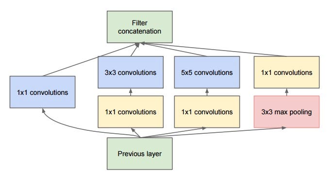Inception Module: The Building Block of the Inception CNN

All of the Python code for this project is in a Jupyter Notebook available on my machine learning projects GitHub repository. The Jupyter Notebook should be run from within the Slim folder in the TensorFlow Models GitHub repository that was downloaded in the previous post. This project was adapted from the TensorFlow Slim Walkthrough Jupyter Notebook and aided by the great book Hands-On Machine Learning with Scikit-Learn and Tensorflow by Aurelien Geron. I ran the TensorFlow sessions in the Jupyter Notebook on a 2GB Nvidia GeForce 940M dedicated graphics card on my laptop. The training times reflect the capabilities of my laptop and will vary considerably depending on your hardware. I highly recommend setting up a compute engine using Google Cloud to run the Jupyter Notebook (or other computationally taxing projects) on a cloud server. Google has GPUs available to rent by the compute-minute and provides free credit when you create an account. (I am also looking forward to the public availability of TPUs or Tensor Processing Units that promise to considerably speed up machine learning training).

Labeled Faces in the Wild

Selecting an appropriate dataset is the most important aspect of this project. The dataset needs to contain enough valid labeled images in each class to allow the neural network to learn every label. There is no magic threshold for number of image per class, but more images, so long as they are correctly labeled, will always improve the performance of the model. The ImageNet dataset contains an average of 1200 images per class, which would be prohibitive for training with the resources available to the typical consumer (although this will change as cloud computing resources become ever more ubiquitous and the price of computing power continues to decline). After a bit of research, I decided to forgo the traditional labeled flowers dataset (this is available as part of TensorFlow and forms the basis for the TensorFlow walk-through tutorial on training the Inception CNN for a novel dataset) in favor of the Labeled Faces in the Wild (LFW) dataset. This is a collection of 13000 images of 5749 individuals gathered from the Internet. Using all of the classes (individuals) would result in a useless model because many of the individuals have only a single image. There is no possibility that even the most powerful convolutional neural network (as of the time of this writing) could learn to identify an individual from a single image. In order to give the model a chance to learn all of the classes, I decided to limit the data to only the 10 individuals with the most images in the dataset. This results in 10 classes with at least 50 images in each class.

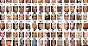Example Images from Labeled Faces in the Wild Dataset

There are several versions of the Labeled Faces in the Wild dataset, with different transformations applied to the images. I choose to use the images that had been processed through deep funneling, a technique of image alignment that seeks to reduce intra-class variability in order to allow the model to learn inter-class differences. Ideally, we want images belonging to the same individual to be similarly aligned so the network learns to differentiate between images based on the face in the image and not the particular orientation of the face, lighting in the image, or background behind the face. The original purpose of the LFW dataset is facial verification, or identifying whether or not two pictures are of the same individual (this could be useful in security applications such as unlocking a door based on one’s face or identifying suspected criminals). Deep funneling was shown to improve the performance of a neural network on image verification. Although we are dealing with image identification, that is, we give the network one image and want to predict the class, image alignment through deep funneling should improve the performance for our task based on the same principles that allow it to work for image verification. Throughout this project, keep in mind that the Inception network has been trained on 1.2 million images of objects and not a single human face. Our task is to train a single layer of the network (out of more than 100 total) to differentiate between 10 different human faces. We are adapting a CNN that has never previously seen a human (‘human’ was not one of the 1000 labels in the ImageNet dataset) to accomplish image identification. The idea that model good for one task are often adept at related problems is a powerful concept in machine learning and the techniques demonstrated in this project are of greater important than the final overall accuracy (although it is fun to be right).

Download the Latest Checkpoint of Pre-Trained Inception Model

We first need to make sure that we have the most up-to-date Inception V3 model with the parameters learned through training on the ImageNet dataset. The following code will download the latest version and extract the required checkpoint:

# Trusty machine learning imports
import tensorflow as tf
import numpy as np

# Make sure to run notebook within slim folder
from datasets import dataset_utils
import os

# Base url
TF_MODELS_URL = "[http://download.tensorflow.org/models/](http://download.tensorflow.org/models/?)"

# Modify this path for a different CNN
INCEPTION_V3_URL = TF_MODELS_URL + "inception_v3_2016_08_28.tar.gz"

# Directory to save model checkpoints
MODELS_DIR = "models/cnn"

INCEPTION_V3_CKPT_PATH = MODELS_DIR + "/inception_v3.ckpt"

# Make the model directory if it does not exist
if not tf.gfile.Exists(MODELS_DIR):
 tf.gfile.MakeDirs(MODELS_DIR)

# Download the appropriate model if haven't already done so
if not os.path.exists(INCEPTION_V3_CKPT_PATH):
 dataset_utils.download_and_uncompress_tarball(INCEPTION_V3_URL, MODELS_DIR)

Inception V3 Schema

Download the Labeled Faces in the Wild Dataset

Once we have the correct model (feel free to adapt this project to a different pre-trained CNN provided by Google) we need to download the full LFW deep-funneled dataset. We will use a similar process to download and extract the dataset to a new directory:

# Full deep-funneled images dataset
FACES_URL = "[http://vis-www.cs.umass.edu/lfw/lfw-deepfunneled.tgz](http://vis-www.cs.umass.edu/lfw/lfw-deepfunneled.tgz?)"
IMAGES_DOWNLOAD_DIRECTORY = "tmp/faces"
IMAGES_DIRECTORY = "images/faces"

if not os.path.exists(IMAGES_DOWNLOAD_DIRECTORY):
 os.makedirs(IMAGES_DOWNLOAD_DIRECTORY)

# If the file has not already been downloaded, retrieve and extract it
if not os.path.exists(IMAGES_DOWNLOAD_DIRECTORY + "/lfw-deepfunneled.tgz"):
 dataset_utils.download_and_uncompress_tarball(FACES_URL, IMAGES_DOWNLOAD_DIRECTORY)

Output:
>> Downloading lfw-deepfunneled.tgz 100.0%
Successfully downloaded lfw-deepfunneled.tgz 108761145 bytes.

The complete deep-funneled dataset is 103 MB. The dataset is structured with a top-level folder called ‘faces’ that contains a number of folders each with the images of a single individual. We now need to work on finding the individuals with the most images. We can use the os Python module to find the number of images total and the number of images of each individual. We will sort the people in the dataset by the number of photos of them and then move them to a new directory. Each folder in the new directory will have all the images for one individual and will be renamed with the number of images and the name of the individual. This should allow us to easily create training, validation, and testing sets.

people_number = []

# Count number of photos of each individual. People number is a list of tuples
# with each tuple composed of the name and the number of photos of a person.
for person in people:
 folder_path = IMAGES_DOWNLOAD_DIRECTORY + '/lfw-deepfunneled/' + person
 num_images = len(os.listdir(folder_path))
 people_number.append((person, num_images))

# Sort the list of tuples by the number of images
people_number = sorted(people_number, key=lambda x: x[1], reverse=True)

# List Comprehension to determine number of people with one image
people_with_one_photo = [(person) for person, num_images in people_number if num_images==1]
print("Individuals with one photo: {}".format(len(people_with_one_photo)))

Output:
Individuals with one photo: 4069

It is a good idea to not use all the images! With 4069 individuals with only a single image, a neural network trained on this dataset would be thoroughly confused by all the different classes (in more technical terms, the bias of the neural network would be too great because it could not actually learn the underlying differences between each class). Now we can create the new directories:

from distutils.dir_util import copy_tree

# Number of individuals to retain
num_classes = 10

# Make the images directory if it does not exist
if not os.path.exists(IMAGES_DIRECTORY):
 os.mkdir(IMAGES_DIRECTORY)

 # Take the ten folders with the most images and move to new directory
 # Rename the folders with the number of images and name of individual
 for person in people_number[:num_classes]:
 name = person[0]
 # Original download directory path
 folder_path = IMAGES_DOWNLOAD_DIRECTORY + '/lfw-deepfunneled/' + name
 formatted_num_images = str(person[1]).zfill(3)
 new_folder_name = "{} {}".format(formatted_num_images, name)
 image_new_name = IMAGES_DIRECTORY + "/" + new_folder_name

 # Make a new folder for each individual in the images directory
 os.mkdir(IMAGES_DIRECTORY + '/' + name)
 # Copy the folder from the download location to the new folder
 copy_tree(folder_path, IMAGES_DIRECTORY + '/' + name)
 # Rename the folder with images and individual
 os.rename(IMAGES_DIRECTORY + '/' + name, image_new_name)

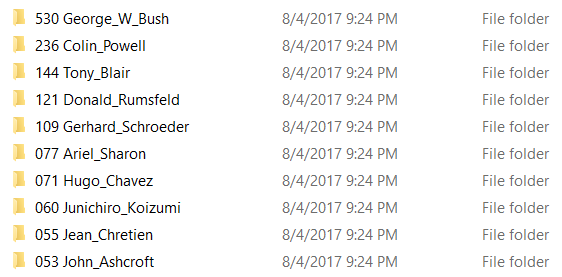Directory with Top 10 Individuals

We can check to make sure that the new directory was correctly created by manual inspection and comparing the new directory to the original.

We have the top-10 individuals by number of photos with the images in an easy-to-access location. We can now split the data into training, validation, and testing datasets with a few basic operations. Unfortunately, we can see right away that we have a limited number of pictures in some of the classes. 50 images may be enough for a human to correctly learn a new face (most of the time one image is sufficient thanks to our extraordinary capacity for facial identification) but it is a relatively small sample when compared to ideal machine learning training sets. We can also see that there is an uneven class distribution with George W. Bush and Colin Powell making up more than half of the images. This is a problem because the CNN might learn to identify these individuals with more photos at the expense of all others. In other words, it might be able to correctly identify every photo of George W. Bush, but it will also incorrectly label many people as Bush who are not because in cases where the network is unsure, the default option could be Bush simply because it has seen more images of Bush. If we were to get many false positives labeled as Bush, we would say that the model has a high recall with respect to Bush — it correctly identifies Bush when it is in him — but it has a low precision — many of the times it claims to see Bush, it is not him. There will always be a tradeoff between precision and recall, and it is up to the developer to adjust the training data and architecture to achieve the correct balance. Maybe we want to create a classifier with a high recall for Tony Blair, and we can tolerate a number of false positives. On the other hand, we might want a classifier that identifies suspected criminals with high precision which would not produce many false positives (false accusations in this case) at the expense of a few false negatives. For now, we will leave the training data as is and see what kind of results we can achieve with a non-optimal dataset.

We need a training set to allow the network to learn the classes, a validation set to implement early stopping when training, and a testing set to evaluate the performance of each model. I will put 70% of each class in a training set, 5% in a validation set, and 25% in a testing set.

# Map each class to an integer label
class_mapping = {}
class_images = {}

# Create dictionary to map integer labels to individuals
# Class_images will record number of images for each class
for index, directory in enumerate(os.listdir("images/faces")):
 class_mapping[index] = directory.split(" ")[1]
 class_images[index] = int(directory.split(' ')[0])

print(class_mapping)

output:
{0: 'John_Ashcroft',
 1: 'Jean_Chretien',
 2: 'Junichiro_Koizumi',
 3: 'Hugo_Chavez',
 4: 'Ariel_Sharon',
 5: 'Gerhard_Schroeder',
 6: 'Donald_Rumsfeld',
 7: 'Tony_Blair',
 8: 'Colin_Powell',
 9: 'George_W_Bush'}

We can also look at the distribution of images in each class:

total_num_images = np.sum(list(class_images.values()))

print("Individual \t Composition of Dataset\n")
for label, num_images in class_images.items():
 print("{:20} {:.2f}%".format(
 class_mapping[label], (num_images / total_num_images) * 100))

output:

Individual Composition of Dataset

John_Ashcroft 3.64%
Jean_Chretien 3.78%
Junichiro_Koizumi 4.12%
Hugo_Chavez 4.88%
Ariel_Sharon 5.29%
Gerhard_Schroeder 7.49%
Donald_Rumsfeld 8.31%
Tony_Blair 9.89%
Colin_Powell 16.21%
George_W_Bush 36.40%

Clearly we have a biased dataset as discussed above. It will be interesting to see the performance of the network on the images of Bush and Powell when testing as compared to the others.

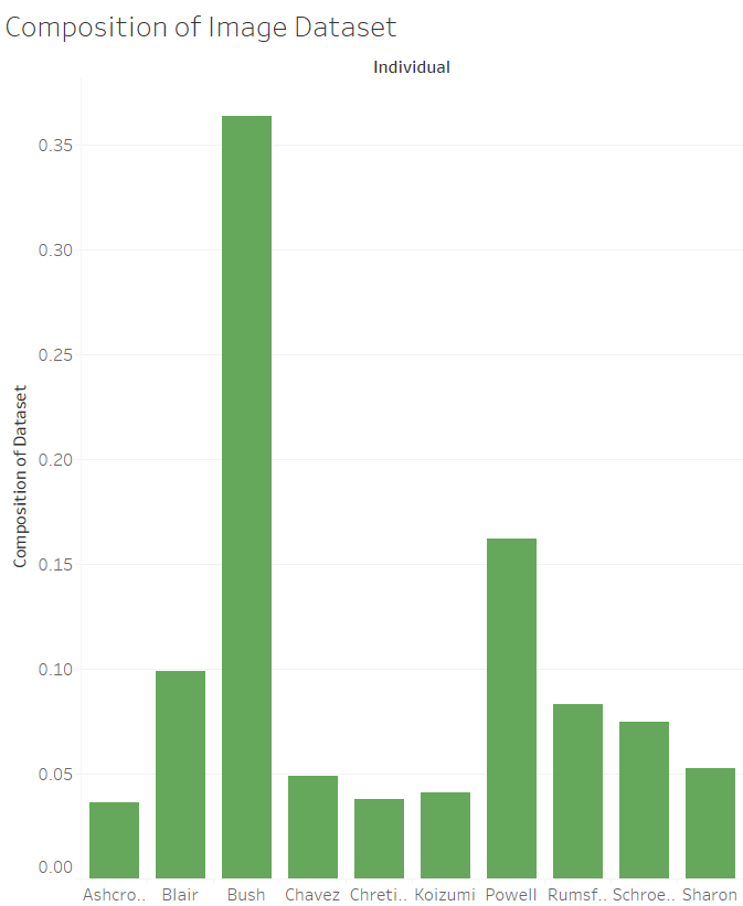Composition of Dataset

The next step is to read the images and labels into arrays that can be split into the three sets. We can use the pyplot module from the matplotlib library to read in the .jpg images as numeric arrays and then convert to numpy arrays:

import matplotlib.pyplot as plt

image_arrays = []
image_labels = []
root_image_directory = "images/faces/"

for label, person in class_mapping.items():
 for directory in os.listdir(root_image_directory):
 if directory.split(" ")[1] == person:
 image_directory = root_image_directory + directory
 break

 for image in os.listdir(image_directory):
 image = plt.imread(os.path.join(image_directory, image))
 image_arrays.append(image)
 image_labels.append(label)

image_arrays = np.array(image_arrays)
image_labels = np.array(image_labels)

print(image_arrays.shape, image_labels.shape)

output:
(1456, 250, 250, 3) (1456,)

Then we will create the set splits with the following code:

import math
from collections import Counter

# Fractions for each dataset
train_frac = 0.70
valid_frac = 0.05
test_frac = 0.25

# This function takes in np arrays of images and labels along with split fractions
# and returns the six data arrays corresponding to each dataset as the appropriate type
def create_data_splits(X, y, train_frac=train_frac, test_frac=test_frac, valid_frac=valid_frac):
 X = np.array(X)
 y = np.array(y)

 # Make sure that the fractions sum to 1.0
 assert (test_frac + valid_frac + train_frac == 1.0), "Test + Valid + Train Fractions must sum to 1.0"

 X_raw_test = []
 X_raw_valid = []
 X_raw_train = []

 y_raw_test = []
 y_raw_valid = []
 y_raw_train = []

 # Randomly order the data and labels
 random_indices = np.random.permutation(len(X))
 X = X[random_indices]
 y = y[random_indices]

 for image, label in zip(X, y):

 # Number of images that correspond to desired fraction
 test_length = math.floor(test_frac * class_images[label])
 valid_length = math.floor(valid_frac * class_images[label])

 # Check to see if the datasets have the right number of labels (and images)
 if Counter(y_raw_test)[label] < test_length:
 X_raw_test.append(image)
 y_raw_test.append(label)
 elif Counter(y_raw_valid)[label] < valid_length:
 X_raw_valid.append(image)
 y_raw_valid.append(label)
 else:
 X_raw_train.append(image)
 y_raw_train.append(label)

 return np.array(X_raw_train, dtype=np.float32), np.array(X_raw_valid, dtype=np.float32), np.array(X_raw_test, dtype=np.float32), np.array(y_raw_train, dtype=np.int32), np.array(y_raw_valid, dtype=np.int32), np.array(y_raw_test, dtype=np.int32)

# Create all the testing splits using the create_splits function
X_train, X_valid, X_test, y_train, y_valid, y_test = create_data_splits(image_arrays, image_labels)

Notice that the datatypes for the images are float pointing numbers and the labels are integers (both with 32 bit precision). Let’s take a look to make sure that the shape of all the arrays looks to be in order:

# Check the number of images in each dataset split
print(X_train.shape, X_valid.shape, X_test.shape)
print(y_train.shape, y_valid.shape, y_test.shape)

output:
(1027, 250, 250, 3) (68, 250, 250, 3) (361, 250, 250, 3)
(1027,) (68,) (361,)

That looks perfectly fine (if a little limited on the amount of training data). The data wrangling step is now complete. Often, this is the most time-intensive and costly part of the entire machine learning workflow. We were using a clean dataset to begin with, which cuts down on data preparation, but it still took a few lines of Python code to create the appropriate datasets.

As a check for accuracy (and for a little bit of fun) we can visualize the images in each class. I have to say, that if this neural network can correctly identify more than 5 of these individuals, then it will outperform me on this task. We can plot 2 images from each class:

# Import matplotlib and use magic command to plot in notebook
import matplotlib.pyplot as plt
%matplotlib inline

# Function to plot an array of RGB values
def plot_color_image(image):
 plt.figure(figsize=(4,4))
 plt.imshow(image.astype(np.uint8), interpolation='nearest')
 plt.axis('off')

import random

# PLot 2 examples from each class
num_examples = 2

# Iterate through the classes and plot 2 images from each
for class_number, person in class_mapping.items():
 print('{} Number of Images: {}'.format(person, class_images[class_number]))
 example_images = []
 while len(example_images) < num_examples:
 random_index = np.random.randint(len(X_train))
 if y_train[random_index] == class_number:
 example_images.append(X_train[random_index])

 for i, image in enumerate(example_images):
 plt.subplot(100 + num_examples*10 + i + 1)
 plt.imshow(image.astype(np.uint8), interpolation='nearest')
 plt.axis('off')
 plt.show()

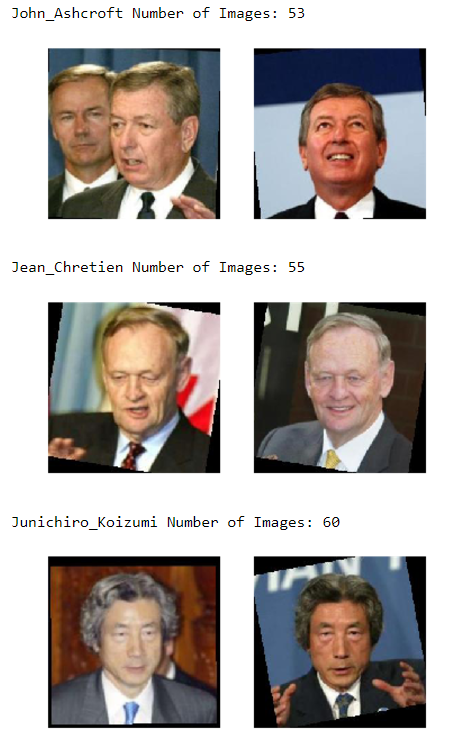
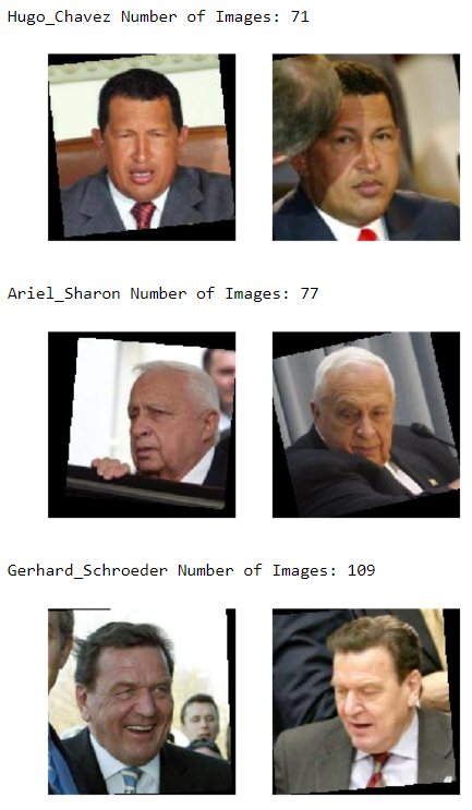Individuals in Image Dataset

(All 15 leaders can be seen in the Jupyter Notebook)

Processing the Images

The ImageNet CNN requires that the images be provided as arrays in the shape [batch_size, image_height, image_width, color_channels]. Batch size is the number of images in a training or testing batch, the image size is 299 x 299 for Inception V3, and the number of color channels is 3 for Red-Green-Blue. In a given color channel, each specific x,y location denotes a pixel with a value between 0 and 255 representing the intensity of the particular color. ImageNet requires that these pixel values are normalized between 0 and 1 which simply means dividing the entire array by 255. Inception has built-in functions for processing an image to the right size and format, but we can also use scipy and numpy to accomplish the same task. All of the images in the LFW data are 255 x 255 x 3 and these will be converted to 299 x 299 x 3 and normalized to pixel values between 0 and 1. The following code accomplishes this processing (which is applied during training):

from scipy.misc import imresize

# Function takes in an image array and returns the resized and normalized array
def prepare_image(image, target_height=299, target_width=299):
 image = imresize(image, (target_width, target_height))
 return image.astype(np.float32) / 255

Define Layer of Inception CNN to Train

In order to adapt the CNN to learn new classes, we must train at least one layer of the network and define a new output layer. We use the parameters that Inception V3 has learned from ImageNet for every layer except the last one before the predictions in the hope that whatever weights and biases are helpful in differentiating objects can also be applied to our facial recognition task. We therefore need to take a look at the structure of the network to determine the trainable layer. Inception has many layers and parameters (about 12 million), but we do not want to attempt to train them all.

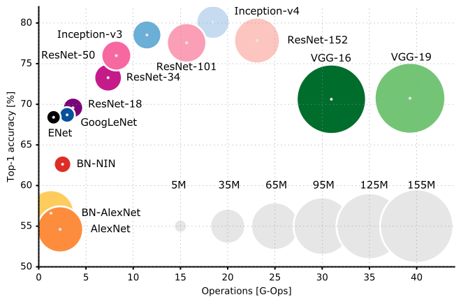Accuracy vs Operations Sized by Parameters for Various CNN Architectures

The inception_v3 function available in the TensorFlow slim library (in the nets folder) returns the unscaled outputs, known as logits, as well as the endpoints, a dictionary with each key containing the outputs from a different layer. If we look at the endpoints dictionary, we can find the final layer before the predictions:

from nets import inception
from tensorflow.contrib import slim

tf.reset_default_graph()

X = tf.placeholder(tf.float32, [None, 299, 299, 3], name='X')
is_training = tf.placeholder_with_default(False, [])

# Run inception function to determine endpoints
with slim.arg_scope(inception.inception_v3_arg_scope()):
 logits, end_points = inception.inception_v3(X, num_classes=1001, is_training=is_training)

# Create saver of network before alterations
inception_saver = tf.train.Saver()

print(end_points)

output:

{'AuxLogits': <tf.Tensor 'InceptionV3/AuxLogits/SpatialSqueeze:0' shape=(?, 1001) dtype=float32>,
 'Conv2d_1a_3x3': <tf.Tensor 'InceptionV3/InceptionV3/Conv2d_1a_3x3/Relu:0' shape=(?, 149, 149, 32) dtype=float32>,
 'Conv2d_2a_3x3': <tf.Tensor 'InceptionV3/InceptionV3/Conv2d_2a_3x3/Relu:0' shape=(?, 147, 147, 32) dtype=float32>,
 'Conv2d_2b_3x3': <tf.Tensor 'InceptionV3/InceptionV3/Conv2d_2b_3x3/Relu:0' shape=(?, 147, 147, 64) dtype=float32>,
 'Conv2d_3b_1x1': <tf.Tensor 'InceptionV3/InceptionV3/Conv2d_3b_1x1/Relu:0' shape=(?, 73, 73, 80) dtype=float32>,
 'Conv2d_4a_3x3': <tf.Tensor 'InceptionV3/InceptionV3/Conv2d_4a_3x3/Relu:0' shape=(?, 71, 71, 192) dtype=float32>,
 'Logits': <tf.Tensor 'InceptionV3/Logits/SpatialSqueeze:0' shape=(?, 1001) dtype=float32>,
 'MaxPool_3a_3x3': <tf.Tensor 'InceptionV3/InceptionV3/MaxPool_3a_3x3/MaxPool:0' shape=(?, 73, 73, 64) dtype=float32>,
 'MaxPool_5a_3x3': <tf.Tensor 'InceptionV3/InceptionV3/MaxPool_5a_3x3/MaxPool:0' shape=(?, 35, 35, 192) dtype=float32>,
 'Mixed_5b': <tf.Tensor 'InceptionV3/InceptionV3/Mixed_5b/concat:0' shape=(?, 35, 35, 256) dtype=float32>,
 'Mixed_5c': <tf.Tensor 'InceptionV3/InceptionV3/Mixed_5c/concat:0' shape=(?, 35, 35, 288) dtype=float32>,
 'Mixed_5d': <tf.Tensor 'InceptionV3/InceptionV3/Mixed_5d/concat:0' shape=(?, 35, 35, 288) dtype=float32>,
 'Mixed_6a': <tf.Tensor 'InceptionV3/InceptionV3/Mixed_6a/concat:0' shape=(?, 17, 17, 768) dtype=float32>,
 'Mixed_6b': <tf.Tensor 'InceptionV3/InceptionV3/Mixed_6b/concat:0' shape=(?, 17, 17, 768) dtype=float32>,
 'Mixed_6c': <tf.Tensor 'InceptionV3/InceptionV3/Mixed_6c/concat:0' shape=(?, 17, 17, 768) dtype=float32>,
 'Mixed_6d': <tf.Tensor 'InceptionV3/InceptionV3/Mixed_6d/concat:0' shape=(?, 17, 17, 768) dtype=float32>,
 'Mixed_6e': <tf.Tensor 'InceptionV3/InceptionV3/Mixed_6e/concat:0' shape=(?, 17, 17, 768) dtype=float32>,
 'Mixed_7a': <tf.Tensor 'InceptionV3/InceptionV3/Mixed_7a/concat:0' shape=(?, 8, 8, 1280) dtype=float32>,
 'Mixed_7b': <tf.Tensor 'InceptionV3/InceptionV3/Mixed_7b/concat:0' shape=(?, 8, 8, 2048) dtype=float32>,
 'Mixed_7c': <tf.Tensor 'InceptionV3/InceptionV3/Mixed_7c/concat:0' shape=(?, 8, 8, 2048) dtype=float32>,
 **'PreLogits': <tf.Tensor 'InceptionV3/Logits/Dropout_1b/cond/Merge:0' shape=(?, 1, 1, 2048) dtype=float32>,**
 'Predictions': <tf.Tensor 'InceptionV3/Predictions/Reshape_1:0' shape=(?, 1001) dtype=float32>}

The ‘PreLogits’ layer is exactly what we are looking for. The size of this layer is [None, 1, 1, 2048] so there are 2048 filters each with size 1 x 1. This layer is created as a result of applying an average pooling operation with an 8 x 8 kernel to the Mixed layers and then applying dropout. We can change this to a fully connected layer by eliminating (squeezing) the two dimensions that are 1, leaving us with a fully connected layer with 2048 neurons. We then create a new output layer that takes the prelogits as input with the number of neurons corresponding to the number of classes. To train only a single layer, we specify the list of trainable variables in the training operation. What the network is learning during training is the connection weights between the 2048 neurons in the prelogits layer and the 10 output neurons as well as the bias for each of the output neurons. We also apply a softmax activation function to the logits returned by the network in order to calculate probabilities for each class:

# Isolate the trainable layer
prelogits = tf.squeeze(end_points['PreLogits'], axis=[1,2])

# Define the training layer and the new output layer
n_outputs = len(class_mapping)
with tf.name_scope("new_output_layer"):
 people_logits = tf.layers.dense(prelogits, n_outputs, name="people_logits")
 probability = tf.nn.softmax(people_logits, name='probability')

# Placeholder for labels
y = tf.placeholder(tf.int32, None)

# Loss function and training operation
# The training operation is passed the variables to train which includes only the single layer
with tf.name_scope("train"):
 xentropy = tf.nn.sparse_softmax_cross_entropy_with_logits(logits=people_logits, labels=y)
 loss = tf.reduce_mean(xentropy)
 optimizer = tf.train.AdamOptimizer(learning_rate=0.01)
 # Single layer to be trained
 train_vars = tf.get_collection(tf.GraphKeys.TRAINABLE_VARIABLES, scope="people_logits")
 # The variables to train are passed to the training operation
 training_op = optimizer.minimize(loss, var_list=train_vars)

# Accuracy for network evaluation
with tf.name_scope("eval"):
 correct = tf.nn.in_top_k(predictions=people_logits, targets=y, k=1)
 accuracy = tf.reduce_mean(tf.cast(correct, tf.float32))

# Intialization function and saver
with tf.name_scope("init_and_saver"):
 init = tf.global_variables_initializer()
 saver = tf.train.Saver()

After isolating the single layer to train, the rest of the code is fairly straightforward and typical for a neural network used for classifcation. We use average cross entropy as a loss function and use the Adam Optimization function with a learning rate of 0.01. The accuracy function will measure top-1 accuracy. Finally, we use an initializer and a saver so that we will be able to save the model during training and restore it at a later time.

Batch Image Processing

During training, we will be passing batches of images to the network. To create these batches, we can write a function that will apply the processing function previously defined at runtime.

# Function takes in an array of images and labels and processes the images to create
# a batch of a given size
def create_batch(X, y, start_index=0, batch_size=4):

 stop_index = start_index + batch_size
 prepared_images = []
 labels = []

 for index in range(start_index, stop_index):
 prepared_images.append(prepare_image(X[index]))
 labels.append(y[index])

 # Combine the images into a single array by joining along the 0th axis
 X_batch = np.stack(prepared_images)
 # Combine the labels into a single array
 y_batch = np.array(labels, dtype=np.int32)

 return X_batch, y_batch

This function will create the training and testing batches at runtime. However, for early stopping, we will be passing all the validation examples through the network at once, so we can go ahead and process the entire validation set:

X_valid, y_valid = create_batch(X_valid, y_valid, 0, len(X_valid))
print(X_valid.shape, y_valid.shape)

output:
(68, 299, 299, 3) (68,)

The validation set is now ready to use for early stopping and we can use this function to create training batches during training (we cannot pass all of the training or testing examples through at once because of the limited amount of memory on the GPU, but the 68 validation examples can fit in memory).

TensorBoard Visualization Operations

TensorBoard is an extremely vital tool for visualizing the structure of the network, the training curves, the images passed to the network, the weights and biases evolution over training, and a number of other features of the network. This information can guide training and optimization of the network. We will stick to relatively basic features of TensorBoard such as looking at the structure of the network, and recording the training accuracy, validation accuracy, and validation loss. We will use the date and time at the start of each training run to create a new TensorBoard log file:

with tf.name_scope("tensorboard_writing"):
 # Track validation accuracy and loss and training accuracy
 valid_acc_summary = tf.summary.scalar(name='valid_acc', tensor=accuracy)
 valid_loss_summary = tf.summary.scalar(name='valid_loss', tensor=loss)
 train_acc_summary = tf.summary.scalar(name='train_acc', tensor=accuracy)

# Merge the validation stats
 valid_merged_summary = tf.summary.merge(inputs=[valid_acc_summary, valid_loss_summary])

# Use the time to differentiate the different training sessions
from datetime import datetime
import time
# Specify the directory for the FileWriter
now = datetime.now().strftime("%Y%m%d_%H%M%S")
model_dir = "{}_unaugmented".format(now)
logdir = "tensorboard/faces/" + model_dir
file_writer = tf.summary.FileWriter(logdir=logdir, graph=tf.get_default_graph())

When we want to look at the statistics, we can run TensorBoard from Windows Powershell (or the command prompt) by navigating to the directory and typing:

C:\Users\Will Koehrsen\Machine-Learning-Projects\pre trained models\slim> tensorboard --logdir=tensorboard/faces

Before we start training, let’s take a look at the computational graph of the Inception V3 CNN.

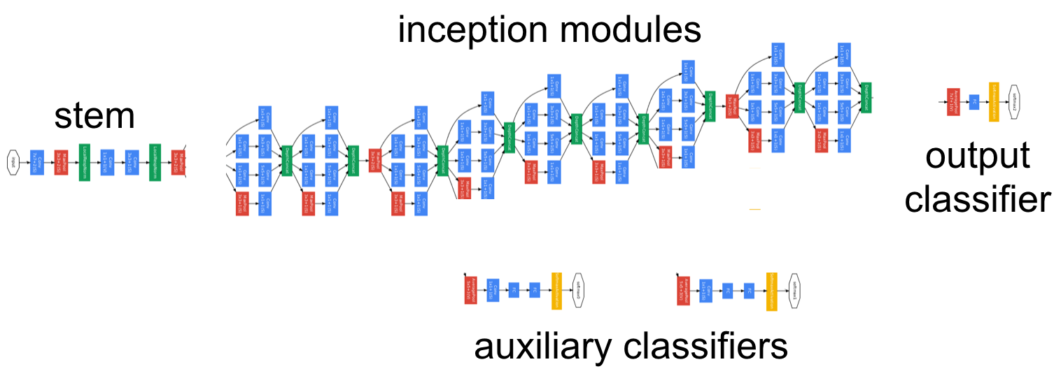
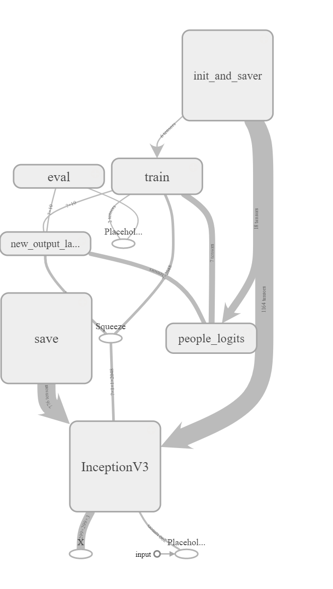*Overall Architecture of Inception CNN

The above figure shows the entire model with each name scope enclosed in a different node. Any of the nodes can be expanded to view the details. For example, here is the expanded new output layer:

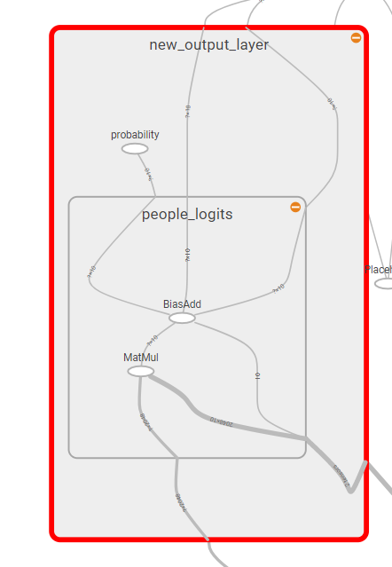Expanded New Output Layer

Here is the expanded Inception V3 node:

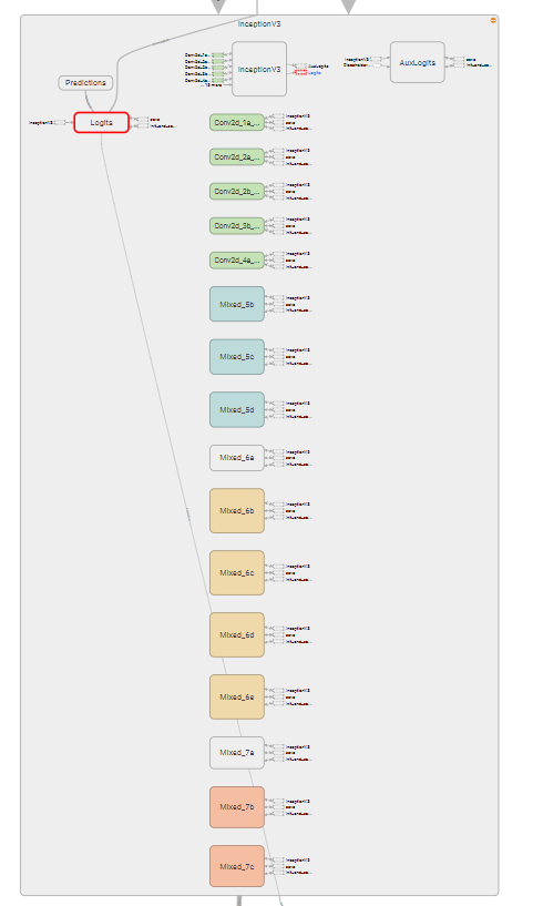Expanded Inception V3 Node

While these computational graphs can be difficult to parse, they contain useful information about the inputs and outputs flowing through the graph. Using namespaces allows us to create a more readable graph and if we wanted to develop our own CNN, the visualization tools available with TensorBoard would be invaluable (see TensorBoard embedding below). Later in this project, we will use TensorBoard to examine the training curves to compare different data augmentation methods.

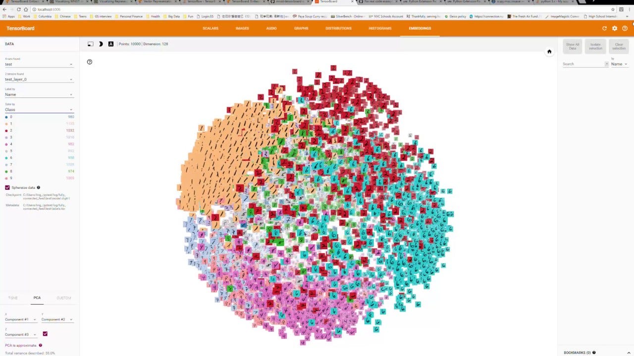TensorBoard Embedding

Training

Finally, we are ready to train the neural network (or at least one layer) for our facial recognition task. We will train using early stopping, which is one method for reducing overfitting on the training set (having too high of a variance). Early stopping requires periodically testing the network on a validation set to assess the score on the cost function (in this case average cross entropy). If the loss does not decrease for a specified number of epochs, training is halted. In order to retain the optimal model, each time the loss improves, we save that model. Then, at the very end of training, we can restore the model that achieved the best loss on the validation set. Without early stopping, the model continues to learn the training set better with each epoch but at the cost of generalization to new instances. There are many implementations of early stopping, but we will use a single validation set and stop training if the loss does not improve for 20 epochs. Each time we run a different model, we will create a new TensorBoard file and save the model parameters to restore for evaluation:

n_epochs = 100
batch_size = 32

# Early stopping parameters
max_checks_without_progress = 20
checks_without_progress = 0
best_loss = np.float("inf")

# Show progress every show_progress epochs
show_progress = 1

# Want to iterate through the entire training set every epoch
n_iterations_per_epoch = len(X_train) // batch_size

# Specify the directory for the FileWriter
now = datetime.now().strftime("%Y%m%d_%H%M%S")
model_dir = "{}_unaugmented".format(now)
logdir = "tensorboard/faces/" + model_dir
file_writer = tf.summary.FileWriter(logdir=logdir, graph=tf.get_default_graph())

# This is the pre-trained model checkpoint training path
inception_v3_checkpoint_path = "models/cnn/inception_v3.ckpt"

# This is the checkpoint path for our trained model with no dataaugmentation
unaugmented_training_path = "models/cnn/inception_v3_faces_unaugmented.ckpt"

with tf.Session() as sess:
 init.run()
 # Restore all the weights from the original CNN
 inception_saver.restore(sess, inception_v3_checkpoint_path)

 t0 = time.time()
 for epoch in range(n_epochs):
 start_index = 0
 # Each epoch, iterate through all the training instances
 for iteration in range(n_iterations_per_epoch):
 X_batch, y_batch = create_batch(X_train, y_train, start_index, batch_size)
 # Train the trainable layer
 sess.run(training_op, {X: X_batch, y: y_batch})
 start_index += batch_size

 # Display the progress of training and write to the TensorBoard directory
 # for later visualization of the training
 if epoch % show_progress == 0:
 train_summary = sess.run(train_acc_summary, {X: X_batch, y: y_batch})
 file_writer.add_summary(train_summary, (epoch+1))
 #Size for validation limited by GPU memory (68 images will work)
 valid_loss, valid_acc, valid_summary = sess.run([loss, accuracy, valid_merged_summary], {X: X_valid, y: y_valid})
 file_writer.add_summary(valid_summary, (epoch+1))
 print('Epoch: {:4} Validation Loss: {:.4f} Accuracy: {:4f}'.format(
 epoch+1, valid_loss, valid_acc))

 # Check to see if network is still improving, if improved during epoch
 # a snapshot of the model will be saved to retain the best model
 if valid_loss < best_loss:
 best_loss = valid_loss
 checks_without_progess = 0
 save_path = saver.save(sess, unaugmented_training_path)

 # If network is not improving for a specified number of epochs, stop training
 else:
 checks_without_progress += 1
 if checks_without_progress > max_checks_without_progress:
 print('Stopping Early! Loss has not improved in {} epochs'.format(
 max_checks_without_progress))
 break

 t1 = time.time()

print('Total Training Time: {:.2f} minutes'.format( (t1-t0) / 60))

The training code produces the following output:

output:
INFO:tensorflow:Restoring parameters from models/cnn/inception_v3.ckpt
Epoch: 1 Validation Loss: 1.5990 Accuracy: 0.529412
Epoch: 2 Validation Loss: 1.4184 Accuracy: 0.632353
Epoch: 3 Validation Loss: 1.2879 Accuracy: 0.573529
Epoch: 4 Validation Loss: 1.2286 Accuracy: 0.632353
Epoch: 5 Validation Loss: 1.2880 Accuracy: 0.573529
Epoch: 6 Validation Loss: 1.5739 Accuracy: 0.455882
Epoch: 7 Validation Loss: 1.9480 Accuracy: 0.500000
Epoch: 8 Validation Loss: 1.7751 Accuracy: 0.441176
Epoch: 9 Validation Loss: 1.3545 Accuracy: 0.558824
Epoch: 10 Validation Loss: 1.3300 Accuracy: 0.544118
Epoch: 11 Validation Loss: 1.7363 Accuracy: 0.514706
Epoch: 12 Validation Loss: 2.1920 Accuracy: 0.323529
Epoch: 13 Validation Loss: 1.4529 Accuracy: 0.558824
Epoch: 14 Validation Loss: 1.8442 Accuracy: 0.455882
Epoch: 15 Validation Loss: 2.6073 Accuracy: 0.485294
Epoch: 16 Validation Loss: 2.7186 Accuracy: 0.485294
Epoch: 17 Validation Loss: 1.7915 Accuracy: 0.588235
Epoch: 18 Validation Loss: 1.7529 Accuracy: 0.632353
Epoch: 19 Validation Loss: 1.4010 Accuracy: 0.676471
Epoch: 20 Validation Loss: 1.3270 Accuracy: 0.661765
Epoch: 21 Validation Loss: 1.3931 Accuracy: 0.632353
Epoch: 22 Validation Loss: 1.4594 Accuracy: 0.705882
Epoch: 23 Validation Loss: 1.8463 Accuracy: 0.647059
Epoch: 24 Validation Loss: 1.7570 Accuracy: 0.691176
Epoch: 25 Validation Loss: 2.4928 Accuracy: 0.558824
Stopping Early! Loss has not improved in 20 epochs
Total Training Time: 38.70 minutes

We already can learn quite a bit from this information. The loss on the validation set was at a minimum on the 5th epoch, and the remaining epochs did nothing to improve the performance of the network. Therefore, we probably do not need to train for so long, but as we are using early stopping, at least the model saved will be the one with the highest performance. We can also see that training took nearly 40 minutes.

Evaluate Performance

Once we have trained the neural network, we need to see if it has any usefulness. To do this, we will evaluate against the test set, which the model has never before seen. As in training, we will go through the test set on batch at a time:

eval_batch_size = 32
n_iterations = len(X_test) // eval_batch_size

with tf.Session() as sess:
 # Restore the new trained model
 saver.restore(sess, unaugmented_training_path)

 start_index = 0
 # Create a dictionary to store all the accuracies
 test_acc = {}

 t0 = time.time()
 # Iterate through entire testing set one batch at a time
 for iteration in range(n_iterations):
 X_test_batch, y_test_batch = create_batch(X_test, y_test, start_index, batch_size=eval_batch_size)
 test_acc[iteration] = accuracy.eval({X: X_test_batch, y:y_test_batch})
 start_index += eval_batch_size

print('Iteration: {} Batch Testing Accuracy: {:.2f}%'.format(
 iteration+1, test_acc[iteration] * 100))

 t1 = time.time()

 # Final accuracy is mean of each batch accuracy
 print('\nFinal Testing Accuracy: {:.4f}% on {} instances.'.format(
 np.mean(list(test_acc.values())) * 100, len(X_test)))
 print('Total evaluation time: {:.4f} seconds'.format((t1-t0)))

The testing code produces the following output:

output:

INFO:tensorflow:Restoring parameters from models/cnn/inception_v3_faces_unaugmented.ckpt
Iteration: 1 Batch Testing Accuracy: 65.62%
Iteration: 2 Batch Testing Accuracy: 68.75%
Iteration: 3 Batch Testing Accuracy: 53.12%
Iteration: 4 Batch Testing Accuracy: 59.38%
Iteration: 5 Batch Testing Accuracy: 62.50%
Iteration: 6 Batch Testing Accuracy: 68.75%
Iteration: 7 Batch Testing Accuracy: 68.75%
Iteration: 8 Batch Testing Accuracy: 71.88%
Iteration: 9 Batch Testing Accuracy: 59.38%
Iteration: 10 Batch Testing Accuracy: 62.50%
Iteration: 11 Batch Testing Accuracy: 46.88%

Final Testing Accuracy: 62.5000% on 361 instances.
Total evaluation time: 30.0208 seconds

Our first attempt at facial recognition correctly identified 62% of individuals. That is by no means impressive for any machine learning system (even if it might outperform most humans) but it at least shows that the network did in fact learn during training. Luckily, if we are not satisfied with this performance, there are a number of steps that we can take in order to improve the neural network that do not involve building our own CNN.

Data Augmentation

The next step is to aim for higher accuracy. The approach we will employ will not modify the neural network itself, but rather will work to expand the dataset. There are two main approaches to augment or increase the amount of training data. The first is simply to gather more labeled training images. That can be time intensive and quite tedious, but as long as the images are valid, it will improve the performance of a machine learning system. Fortunately, there is another approach known as data augmentation. For images, this means taking the existing pictures and applying various shifts that do not alter the identifiable features in the image but rather the presentation of the features. For example, the location of a face within an image should not matter, only the face itself is important for identification. Therefore, if we take one image and shift the face in the image to many locations, we can make the network robust to changes in face location. Likewise, we can rotate the face to make the network invariant to changes in orientation of features. In effect, we are creating a network that is invariant to manipulations of the presentation of the images and only learns to differentiate the faces themselves. Other transformations include altering the background of the images or the lighting or contrast of images to force the network to learn the features in the image and not superfluous differences. We take the existing images, apply a transformation, append the transformed images to the original images with the correct label, and then train the network on the expanded dataset.

Shifting Images

The first transformation to implement will shift the image in four directions (left, right, down, up). TensorFlow has plenty of operations for data augmentation of images, but because we will perform fairly simple transformations, we can use scipy and numpy. The following code applies the four shifts to the images:

import scipy

# Take in an image as an array and return image with a [dx, dy] shift
def shift_image(image_array, shift):
 return scipy.ndimage.interpolation.shift(image_array, shift, cval=0)

# Four shifts of 30 pixels
shifts = [[30,0], [-30,0], [0, 30], [0,-30]]
shifted_images = []
shifted_labels = []

# Iterate through all training images
for image, label in zip(X_train, y_train):

 # Swap the color channel and height axis
 layers = np.swapaxes(image, 0, 2)

 # Apply four shifts to each original image
 for shift in shifts:
 transposed_image_layers = []

 # Apply the shift to the image one layer at a time
 # Each layer is an RGB color channel
 for layer in layers:
 transposed_image_layers.append(shift_image(layer, shift))

 # Stack the RGB layers to get one image and reswap the axes
 transposed_image = np.stack(transposed_image_layers)
 transposed_image = np.swapaxes(transposed_image, 0, 2)

 # Add the shifted images and the labels to a list
 shifted_images.append(transposed_image)
 shifted_labels.append(label)

# Convert the images and labels to numpy arrays
shifted_images = np.array(shifted_images)
shifted_labels = np.array(shifted_labels)

print(shifted_images.shape,shifted_labels.shape)

output:
(4108, 250, 250, 3) (4108,)

We can then visualize the transformation:

ex_index = 5

# Plot original image
plot_color_image(X_train[ex_index])
plt.title("Original Image of {}".format(class_mapping[y_train[ex_index]]))
plt.show()

ex_shifted_images = shifted_images[ex_index*4:(ex_index*4)+ 4]

# Plot four shifted images
for i, image in enumerate(ex_shifted_images):
 shift = shifts[i]
 plt.subplot(2,2,i+1)
 plt.imshow(image.astype(np.uint8), interpolation='nearest')
 plt.title('Shift: {}'.format(shift))
 plt.axis('off')
plt.show()

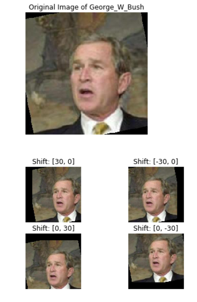Result of Shift Transformation

As you can see, the facial content of the image has not been altered, but the location of the face in the image has been changed. In theory, this will make the network robust to changes in facial location within an image. Finally, we need to append the transformed images to the original training set:

# Create a new training set with the original and shifted images
X_train_exp = np.concatenate((shifted_images, X_train))
y_train_exp = np.concatenate((shifted_labels, y_train))

print(X_train_exp.shape, y_train_exp.shape)

output:
(5135, 250, 250, 3) (5135,)

The end result of this process is a 5x larger training set. Now, we can use the same training and evaluation process to see if our data augmentation procedure had a positive effect.

Training on Augmented Data

We will first train with the augmented data on a clean version of the pre-trained model. The results are below (code to train the model is almost the same as the un-augmented training and can be found in the Jupyter Notebook):

output:
INFO:tensorflow:Restoring parameters from models/cnn/inception_v3.ckpt
Epoch: 1 Validation Loss: 1.1123 Accuracy: 0.573529
Epoch: 2 Validation Loss: 0.9927 Accuracy: 0.617647
Epoch: 3 Validation Loss: 1.0175 Accuracy: 0.602941
Epoch: 4 Validation Loss: 0.9210 Accuracy: 0.661765
Epoch: 5 Validation Loss: 0.9502 Accuracy: 0.676471
Epoch: 6 Validation Loss: 1.0442 Accuracy: 0.705882
Epoch: 7 Validation Loss: 1.3256 Accuracy: 0.647059
Epoch: 8 Validation Loss: 1.4516 Accuracy: 0.647059
Epoch: 9 Validation Loss: 1.1426 Accuracy: 0.632353
Epoch: 10 Validation Loss: 1.1084 Accuracy: 0.661765
Epoch: 11 Validation Loss: 1.1072 Accuracy: 0.720588
Epoch: 12 Validation Loss: 1.4951 Accuracy: 0.661765
Epoch: 13 Validation Loss: 1.0699 Accuracy: 0.691177
Epoch: 14 Validation Loss: 1.1920 Accuracy: 0.691177
Epoch: 15 Validation Loss: 1.3776 Accuracy: 0.676471
Epoch: 16 Validation Loss: 1.8172 Accuracy: 0.632353
Epoch: 17 Validation Loss: 1.6500 Accuracy: 0.617647
Epoch: 18 Validation Loss: 1.1445 Accuracy: 0.720588
Epoch: 19 Validation Loss: 1.4750 Accuracy: 0.617647
Epoch: 20 Validation Loss: 1.1172 Accuracy: 0.720588
Epoch: 21 Validation Loss: 1.3523 Accuracy: 0.750000
Epoch: 22 Validation Loss: 1.3562 Accuracy: 0.676471
Epoch: 23 Validation Loss: 1.5062 Accuracy: 0.691177
Epoch: 24 Validation Loss: 1.2096 Accuracy: 0.720588
Stopping Early! Loss has not improved in 20 epochs
Total Training Time: 166.66 minutes

The training time did significantly increase because of the larger number of training examples. The following output shows the result of evaluation on the test set:

output:
INFO:tensorflow:Restoring parameters from models/cnn/inception_v3_faces_augmented.ckpt
Iteration: 1 Batch Testing Accuracy: 68.75%
Iteration: 2 Batch Testing Accuracy: 65.62%
Iteration: 3 Batch Testing Accuracy: 81.25%
Iteration: 4 Batch Testing Accuracy: 71.88%
Iteration: 5 Batch Testing Accuracy: 78.12%
Iteration: 6 Batch Testing Accuracy: 68.75%
Iteration: 7 Batch Testing Accuracy: 75.00%
Iteration: 8 Batch Testing Accuracy: 78.12%
Iteration: 9 Batch Testing Accuracy: 71.88%
Iteration: 10 Batch Testing Accuracy: 81.25%
Iteration: 11 Batch Testing Accuracy: 59.38%

Final Augmented with Clean Start Testing Accuracy: 72.7273% on 361 instances.
Evaluation Time: 28.73 seconds

Well, that made quite a difference! Our accuracy jumped from 62.5% to 72.7%, a relative improvement of 16%. However, we did pay for it with a greater than 400% increase in training time. In the real world, we would need to weigh the training time versus performance with a cost-benefit analysis to determine the acceptable balance between accuracy and development time.

Another approach we can use is to train using the augmented dataset but start from the best checkpoint saved by the un-augmented model. This should speed up training and could result in a performance boost as well. The idea is that the parameters will need less training to converge to their optimal values than starting with a clean pre-trained model. To implement this, we will simply change the checkpoint path that we initialize the parameters with:

restart_augmented_training_path = "models/cnn/inception_v3_faces_restart_augmented.ckpt"

with tf.Session() as sess:
 init.run()
 inception_saver.restore(sess, unaugmented_training_path)

The rest of the training code is the same. We can then again evaluate on the test set:

output:
Final Augmented with Restart Testing Accuracy: 73.8636% on 361 instances.

Starting from the un-augmented checkpoint did not reduce training time (167 minutes versus 166 minutes for the clean start) but it did result in a 1.6% relative improvement in accuracy. Again, there are any number of data augmentation methods we could try, and we are only limited by time and computing power. I will try one more simple data augmentation.

Flipping Images

Another straightforward image transformation is to flip the content of the image from left to right. Imagine this as placing a mirror vertically dividing the image in two and mapping the left to the right side and the right side to the left side (perhaps that is a bad explanation. If so, scroll to the photos below). This preserves the facial content of the images but alters the orientation, again with the purpose of making the network invariant to the presentation of the face within the image. The following code flips the images from left to right:

images_flipped = []
labels_flipped = []

# Flip every image in the training set
for image, label in zip(X_train, y_train):
 images_flipped.append(np.fliplr(image))
 labels_flipped.append(label)

# Convert the flipped images and labels to arrays
images_flipped = np.array(images_flipped)
labels_flipped = np.array(labels_flipped)

Visualizing the images provides a better context for this transformation than a written explanation:

ex_index = 652

plot_color_image(X_train[ex_index])
plt.title('Original Image of {}'.format(class_mapping[y_train[ex_index]]))
plt.show()

plot_color_image(images_flipped[ex_index])
plt.title('Left to Right Flipped Image')
plt.show()

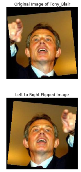Left to Right Flip Transformation

The content of the images has not been altered, only flipped left to right. We then append these flipped images to the original dataset and end up with a 2x larger training set:

X_train_with_flip = np.concatenate((X_train, images_flipped))
y_train_with_flip = np.concatenate((y_train, labels_flipped))

print(X_train_with_flip.shape, y_train_with_flip.shape)

output:
(2054, 250, 250, 3) (2054,)

Training from a clean start results in a 66.2% accuracy and a 70 minute training time. Starting from the best previously saved model results in a 66 minute training time and a 60.5% accuracy. In this case, we achieved a 6% relative increase in accuracy over the un-augmented training set with less than a doubling of training time. In industry, this might be a better trade than the 16% performance increase at the cost of 400% increase in training time that we got from the shifted images augmentation.

While there are any number of additional transformations to try, we are more interested in the process than achieving perfect accuracy. To that end, we can restore the best-performing model — the model trained on the shifted images dataset starting from the un-augmented checkpoint — and look at the results.

Visualizing Performance of the CNN

To look at the results, we create a simple function that prints the correct label, the image, and the ten probabilities corresponding to each class. The function will take in an index to use from the test set. We could use images from the Internet, but the images in the test set have already been deep-funneled and provide an appropriate standard for evaluation because our classifier was not trained on these images. The following code creates the function:

def classify_image(index, images=X_test, labels=y_test):
 image_array = images[index]
 label = class_mapping[labels[index]]

 prepared_image = prepare_image(image_array)
 prepared_image = np.reshape(prepared_image, newshape=(-1, 299, 299, 3))

 with tf.Session() as sess:
 saver.restore(sess, restart_augmented_training_path)
 predictions = sess.run(probability, {X: prepared_image})

 predictions = [(i, prediction) for i, prediction in enumerate(predictions[0])]
 predictions = sorted(predictions, key=lambda x: x[1], reverse=True)
 print('\nCorrect Answer: {}'.format(label))
 print('\nPredictions:')
 for prediction in predictions:
 class_label = prediction[0]
 probability_value = prediction[1]
 label = class_mapping[class_label]
 print("{:26}: {:.2f}%".format(label, probability_value * 100))

 plot_color_image(image_array)
 return predictions

Let’s make some predictions:

predictions = classify_image(20)

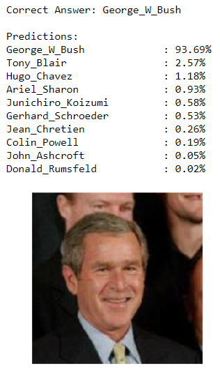Predictions for Bush Test Image

predictions = classify_image(346)

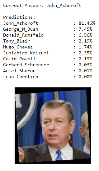Predictions for Ashcroft Test Image

predictions = classify_image(123)

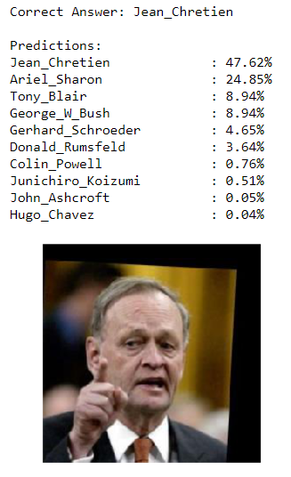Predictions for Chretien Test Image

That’s a pretty decent performances so far. Of course, to correctly represent the 73% testing accuracy, we need to observe that the network is not always correct:

predictions = classify_image(9)

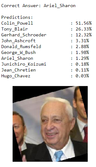Predictions for Sharon Test Image

I would not be surprised if the majority of the wrong classifications were incorrectly labeled as Powell or Bush. The network has seen many more images of these two individuals than any other during training so they could become the default option when the CNN is unsure. If you were classifying faces, and a plurality of the training images belonged to George W Bush, then if you saw an image you were not sure about when you were being tested, the best bet would be to guess Bush because he constituted the largest percentage of the images.

Distribution of Test Predictions

To back up my prior assertion with some data (or to prove it false), we can take a look at all the predictions on the test set to see if Bush and Powell make up more than their fair share of predictions. This requires a slight modification of the testing code to save each set of predictions for later analysis:

eval_batch_size = 32
n_iterations = len(X_test) // eval_batch_size

# Evaluation with saved predictions
with tf.Session() as sess:
 saver.restore(sess, restart_augmented_training_path)

 test_predictions = []
 start_index = 0

 # Add each set of predictions to a list
 for iteration in range(n_iterations):
 X_test_batch, y_test_batch = create_batch(X_test, y_test, start_index, batch_size=eval_batch_size)
 test_predictions.append(probability.eval({X: X_test_batch, y: y_test_batch}))
 start_index += eval_batch_size

# Convert list of predictions to np array
test_predictions = np.array(test_predictions)
test_predictions.shape

output:
(11, 32, 10)

Then we can generate the labels using the argmax function (that returns the index of the maximum value) applied across the first axis (across each row):

# Reshape predictions to correct shape and generate label array
test_predictions = np.reshape(test_predictions, (-1, 10))
test_predictions_label = np.argmax(test_predictions, axis=1)
test_predictions_label.shape

output:
(352,)

Then adjust the test set to match the size of the test predictions (because some of the test set is not used when batches are created):

# A few of the testing examples are left off by the batching process
y_test_eval = y_test[:352]

# Make sure that accuracy agrees with earlier evaluation
test_accuracy = np.mean(np.equal(test_predictions_label, y_test_eval))
print("Test Accuracy: {:.2f}%".format(test_accuracy*100))

output:
Test Accuracy: 73.86%

The test accuracy from manually evaluating is the same as in the TensorFlow session which is a good indication that we correctly stored the predictions. Now we can numerically evaluate the distribution of predictions against the actual distribution of images in the test set:

print('Individual: \t Composition of Test Set \t Composition of Predictions')
total_test_images = len(y_test_eval)

for label, individual in class_mapping.items():
 n_test_images = Counter(y_test_eval)[label]
 n_predictions = Counter(test_predictions_label)[label]
 print("{:26} {:5.2f}% {:26.2f}%".format(
 individual, n_test_images / total_test_images * 100, n_predictions / total_test_images * 100))

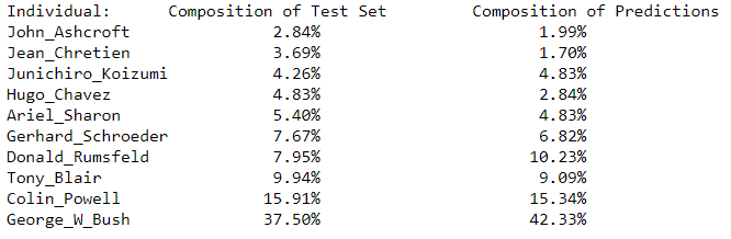Distribution of Test Images and Predictions

We can also show the difference between the test set composition and the prediction composition:

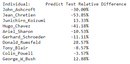Prediction and Test Composition Relative Difference

Individuals with a negative percentage had less predictions from the neural network than they had images in the test set, while individuals with a positive percentage generated more predictions than images in the test set.

My analysis of the performance of the CNN was not entirely accurate. While George W Bush did have more predictions than he should have according to the composition of the test set, Colin Powell actually received fewer predictions than would be expected. From this information, we could generate a confusion matrix and determine the recall and precision for each individual, but this post is already getting long enough as it is! For now, we will settle with a couple graphical distributions to visualize the differences in composition of classes between the test set and predictions. We can start with frequency plots:

# Visualize distribution of images in test set
bins = np.arange(11)
fig, ax = plt.subplots(figsize=(14, 8))
plt.subplots_adjust(wspace=0.25)
plt.subplot(1,2,1)
plt.hist(y_test_eval, bins=bins, lw=1.2, edgecolor='black')
plt.title('Frequency of Classes in Test Set'); plt.xlabel('Class'); plt.ylabel('Count');
names = list(class_mapping.values())
xlabels = [name.split("_")[1] for name in names]
plt.xticks(bins+0.5, xlabels, rotation='vertical');

plt.subplot(1,2,2)
# Visualize distribution of images in predictions
bins = np.arange(11)
plt.hist(test_predictions_label, bins=bins, lw=1.2, edgecolor='black')
plt.title('Frequency of Classes in Predictions'); plt.xlabel('Class'); plt.ylabel('Count');
names = list(class_mapping.values())
xlabels = [name.split("_")[1] for name in names]
plt.xticks(bins+0.5, xlabels, rotation='vertical');

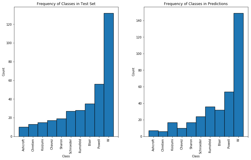Histogram of Class Frequency in Test Set and Predictions

The most revealing graph is the relative difference between the composition of the test set and the predictions:

relative_differences = []

for label, individual in class_mapping.items():
 n_test_images = Counter(y_test_eval)[label]
 n_predictions = Counter(test_predictions_label)[label]
 n_test_pct = n_test_images / total_test_images
 n_predictions_pct = n_predictions / total_test_images

 relative_differences.append((n_predictions_pct - n_test_pct) / n_test_pct * 100)

colors = ['orange' if difference < 0.0 else 'blue' for difference in relative_differences]

# Visualize relative difference in
bins = np.arange(10)
fig, ax = plt.subplots()
plt.bar(bins, relative_differences, lw=1.2, color=colors, edgecolor='black')
plt.title('Relative Differences between Test and Prediction Composition'); plt.xlabel('Class'); plt.ylabel('Relative Difference (%)');
names = list(class_mapping.values())
xlabels = [name.split("_")[1] for name in names]
plt.xticks(bins, xlabels, rotation='vertical');

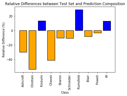Relative Differences between Test Set and Prediction Compositions

There is a large discrepancy between the number of predictions made for some individuals and their representation in the test set. We could say there is a systematic bias towards or against some individuals, but the more likely explanation is that with so few training and testing examples, the relative distributions are mostly chance. If we were to run the training again, we would likely get a significantly different distribution because the model is not able to identify each individual with absolute certainty which results variations across training and evaluation runs.

TensorBoard Training Curves

Finally, if we want to analyze our CNN performance in even greater depth, we can look at the training accuracy, validation loss, and validation accuracy as a function of the epoch for training on the various datasets. This will allow us to see the extent of overfitting (or maybe underfitting) on the training set as well as the effect of data augmentation on the training performance. We kept the statistics relatively simple and did not take advantage of the capabilities of TensorBoard, such as visualizing histograms that show the evolution of weights and biases over the epochs. The full features of TensorBoard (including embedded visualizations) are incredible and are a necessity to use when developing a full CNN or any neural network.

The legend for all of the training runs is below. To summarize, we have five runs defined by the dataset and starting point (with training time and accuracy):

1. Un-augmented data with clean start (38.7 min, 62.5%)
2. Shifted Augmented data with clean start (166.7 min, 72.7%)
3. Shifted Augmented data with restart from un-augmented checkpoint (167.6 min, 73.9%)
4. Flipped Augmented data with clean start (69.2 min, 66.2%)
5. Flipped Augmented data with restart from un-augmented checkpoint (65.8 min, 60.5%)

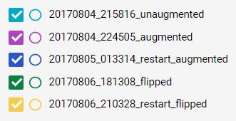Key for Training Curves

The first graph from TensorBoard is the training accuracy:

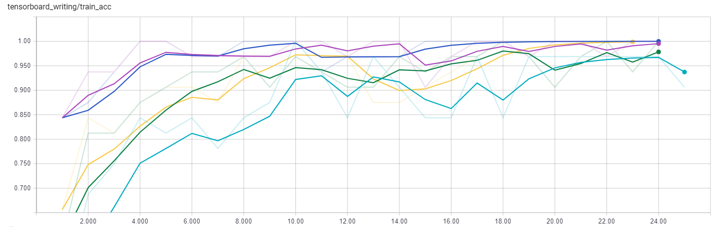Training Accuracy

This is evaluated on a single training batch of 32 instances, so it is not a great indicator of overall performance, but we can see that it training accuracy does increase with number of epochs up to a maximum value with all of the models. Notice that the accuracy ends near 100% which can be a sign of overfitting especially when the validation accuracy is not nearly that high. This is one reason why we chose to implement early stopping so the model could generalize better to new images. Early stopping should reduce the variance of the model, or its sensitivity to training examples allowing it to make better predictions on instances it has never encountered. Early stopping can however increase the bias of a model which is a measure of how closely the algorithm learns the training data. High bias means the neural network essentially overlooks much of the training examples. Training any machine learning model is always an exercise between high variance, which leads to poor generalizations to new instances, and high bias, which prevents the network from learning the underlying relationships during training.

The next curve is the validation loss:

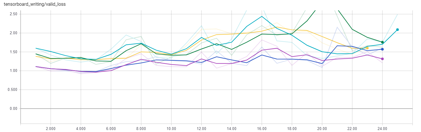Validation Loss

The curve shows that the validation loss does not continually decrease, another sign of overfitting. For all of the training runs, the loss is minimized within the first ten training epochs indicating that further training is unnecessary. The two models trained on the shifted augmented dataset have the lowest validation loss proving that adding shifted images to the training data improved the performance of the network. This is also demonstrated by the validation accuracy curves:

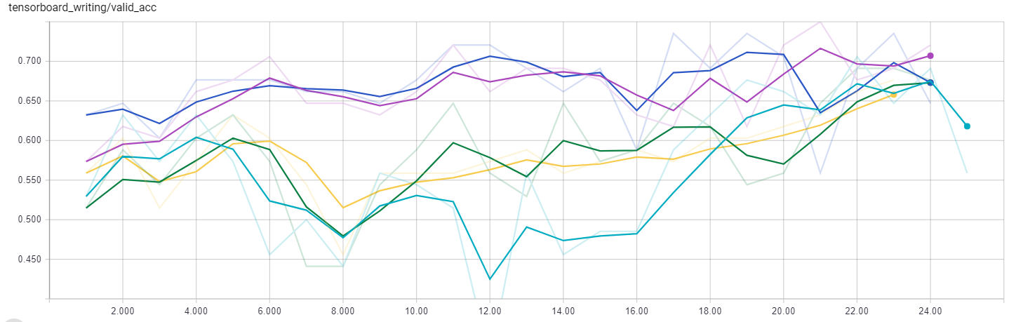Validation Accuracy

These validation accuracy plots clearly show the benefit of augmenting the training data. The lowest performing model in this graph is the un-augmented dataset, followed by the left-to-right flipped dataset, with the shifted dataset, also the largest, on top in terms of accuracy. The validation set is relatively small at 68 images and so will be subject to some variation across runs, but these curves show that we are on the right track with the data augmentation approach and would likely benefit from collecting more labeled training images or performing additional transformations to the existing images. The graphs also show that all of the models achieved the best performance within a handful of epochs. This indicates that we might not need to train the model for as long and we can decrease the number of epochs without a decrease in the loss function required to implement early stopping. Even with simple statistics, the training curves can provide us valuable information about the best strategy for developing a neural network for any task we want to perform.

Conclusion

Rather than an attempt to set a record for facial identification accuracy, this project was more a proof-of-concept to demonstrate the process of training an existing network for a different objective. We were able to take a model pre-trained on a related dataset and adapt it to a task of our choosing. In the process, we were able to save ourselves weeks or even months of development and training time. We saw how we could retain all the parameters of each layer except for the last layer, create a new output layer, and train the single unfrozen layer to achieve adequate performance on facial recognition with a model originally trained to distinguish between 1000 objects. Moreover, we successfully explored the concept of data augmentation by image transformation and we were able to use TensorBoard to understand the computational graph (or at least see the graph) and to observe the training curves which validated our use of data augmentation. There are any number of additional steps to this project that would improve the accuracy. The ones most likely to have a significant impact are to gather more labeled training data or train more layers of the network. Both of these are easy to implement but time-intensive. For now, this project serves to validate the adaption approach for development of a CNN.

This adaptation process is indicative of an industry application in which a company is more likely to use an existing high performance model than start from a clean slate because of the development and training resources required for such a task. Moreover, deep-learning is a collaborative field, where new discoveries necessarily build off previous findings and novel applications for existing neural networks arise out of a mindset of sharing. Great ideas die in isolation, and it is only by collaborating with diverse entities across fields that world-altering innovations can be developed. In that line of thinking, feel free to use, share, and adapt this code in any way you see fit!

Addendum: Who Does the Inception CNN Think I Am?

Predictions for My Image

Originally published at medium.com on August 7, 2017.