(Source)

An Application of the Poisson Process and Poisson Distribution to Model Earth Asteroid Impacts

Here’s some good news: if you’ve spent hours studying a concept by reading books and class notes on the theory and you just can’t seem to get it, there’s a better way to learn. Starting with theory is always difficult and frustrating because you can’t see the most important part of a concept: how it’s used to solve problems. In contrast, learning by doing — working through problems — is more effective because it gives you context, letting you fit the technique into your existing mental framework. Moreover, studying through applications is more enjoyable for those motivated by an intrinsic desire to solve problems.

In this article, we’ll apply the concepts of a Poisson Process and Poisson Distribution to model Earth asteroid impacts. We’ll build on the principles covered in The Poisson Process and Poisson Distribution Explained, putting into practice the ideas with real-world data. Through this project, we’ll get a sense of how to use statistical concepts to solve problems and how to compare the observed results with theoretical expected outcomes.

The full code for this article (with interactive apps) can be run on mybinder.org by clicking the image. The Jupyter Notebook is on GitHub.

Click to launch a Jupyter Notebook on mybinder.org for this article.

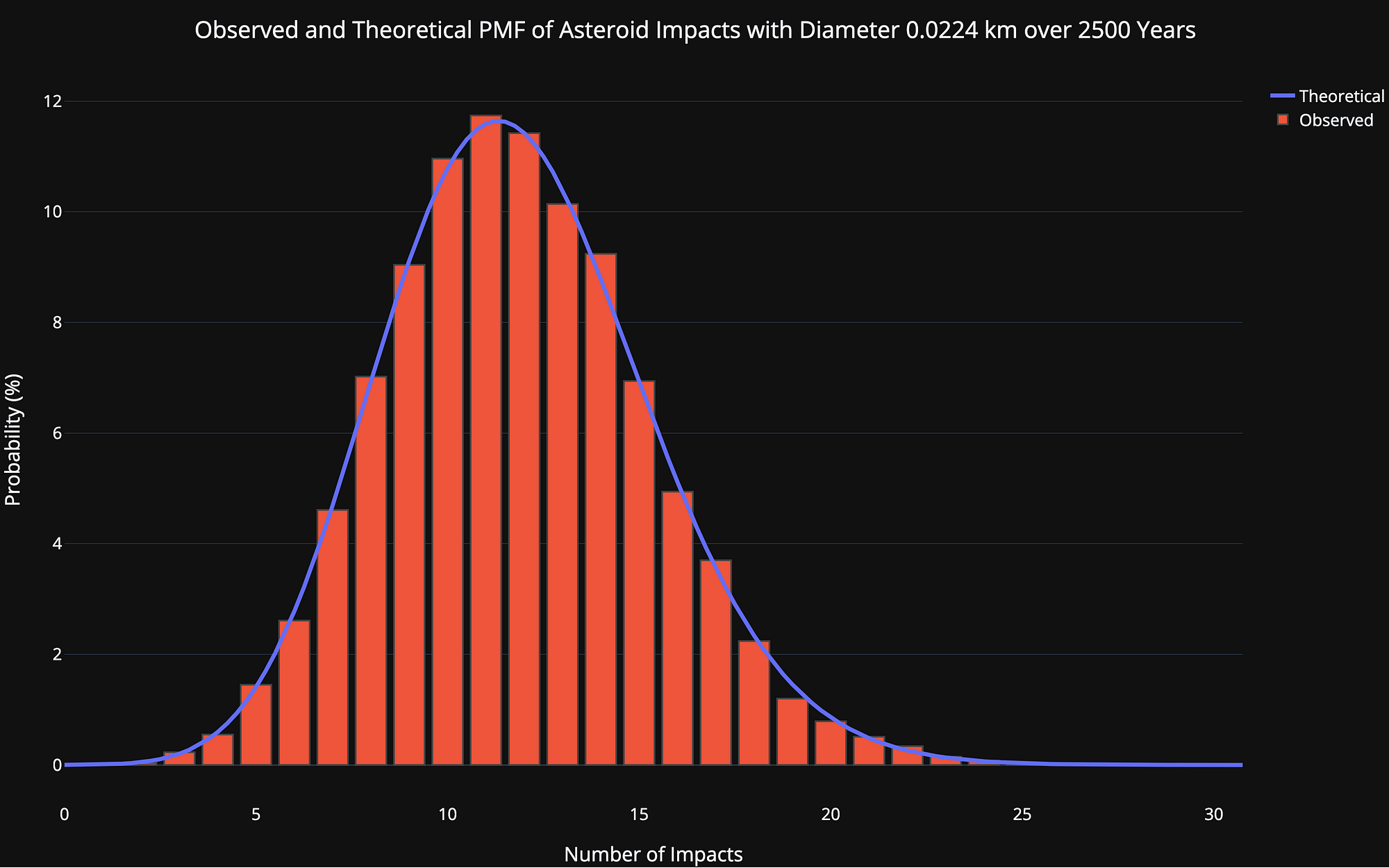Probability Mass Function of Number of Asteroid Impacts

Poisson Process and Poisson Distribution Basics

We won’t cover the full details (see here) but these are the basics we need: The Poisson Process is a model for infrequent events — like asteroid impacts — where we know the average time between events but the actual time between any two events is randomly distributed (stochastic). Each event is independent of all other events, which means we can’t use the time since the last event to predict when the next event will occur. A Poisson model is an extension of a binomial model to situations where the number of expected successes is much less than the number of trials.

Each sub-interval in a Poisson Process is a Bernoulli trial where the event either happens (success) or it does not. In our asteroid example, the event is an asteroid impact and the sub-interval is a year, so each year, an impact either happens or it does not (we’ll assume at most one impact per year and that impacts are independent). Asteroid strikes are — thankfully — infrequent, so the total number of successes is low compared to the number of years (trials) which we’ll consider. Moreover, we know the average time between impacts (we get this from data) but not when exactly the impacts will occur.

To figure out the probability of a number of Poisson Process-generated events occurring in a time interval we use the Poisson Distribution with the Probability Mass Function (PMF):

Poisson Probability Mass Function (PMF) Distribution

Where events/time is a frequency such as impacts/year. This formula is somewhat convoluted so we simplify (events / time) * time to a single parameter, λ. Lambda is the rate parameter of the distribution and is the only parameter we need to define the Poisson:

Poisson PMF

Lambda is the expected (most likely) number of events in the time period. The probabilities of different numbers of events changes as we alter lambda:

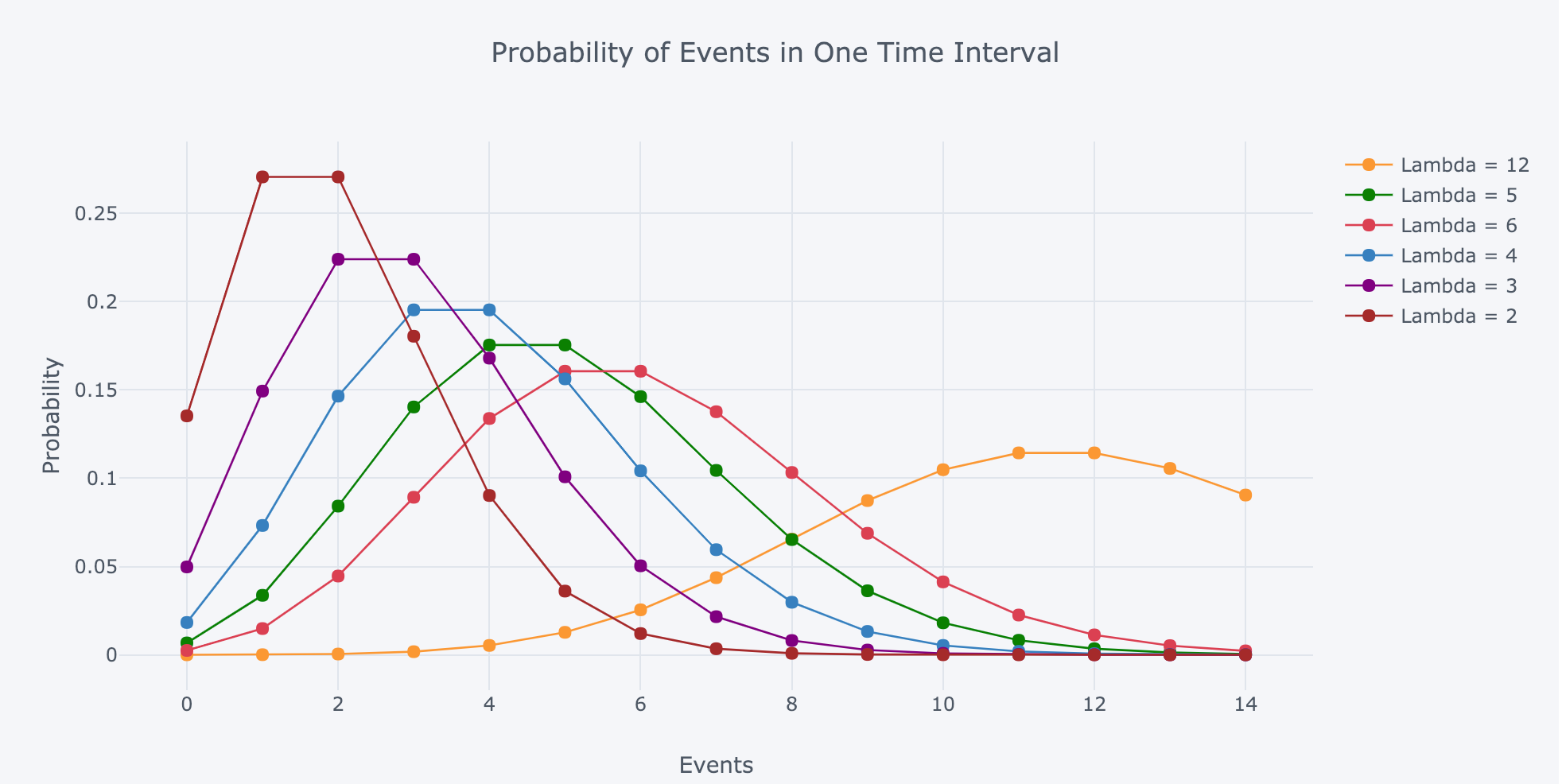Poisson PMF Distribution with differing values of lambda (rate parameter)

Finally, the distribution of time between events (waiting time) is a decaying exponential. The probability of waiting longer than t between events is:

Probability of waiting longer than t in a Poisson process

Waiting times in a Poisson Process are memoryless, meaning they have no dependence on each other. The average waiting time between events works out to be 1 / frequency. The Poisson distribution is fairly simple to wrap your head around as it requires only a single parameter, the rate parameter which is the expected number of events in the interval, or freq * time.

Asteroid Impact Data

To use the Poisson Process and Distribution for asteroid impacts, all we need is the average frequency of asteroid impacts. The bad news is that there is not enough data to pin down the rates precisely. The good news is that scientists have come up with some estimates based on the data we do have (such as the number of Near Earth Asteroids) and robust simulations. We’ll use data in the NASA 2017 Report of the Near Earth Object Science Definition Team which, among tons of fascinating information, provides estimates of the frequency of asteroid impacts for different sized asteroids.

Once we’ve loaded the data and cleaned up the columns, we have this data:

Data from NASA 2017 NEO SDT (5 of the 27 rows)

Each row is a different sized asteroid (with averagediameter in km) and the critical column is the impact_frequency. This gives the average number of impacts per year which we can convert into a time_between_impacts by taking the reciprocal. The impact_frequency decreases with increasing size because there are fewer large asteroids (specified by number).

Although it’s not necessary, I like to start out with data analysis like looking at the impact energy by diameter or the time between impacts by diameter:

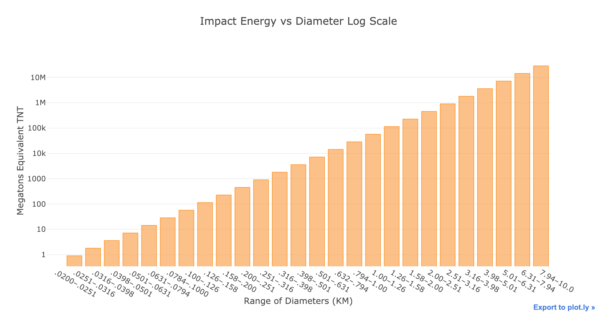
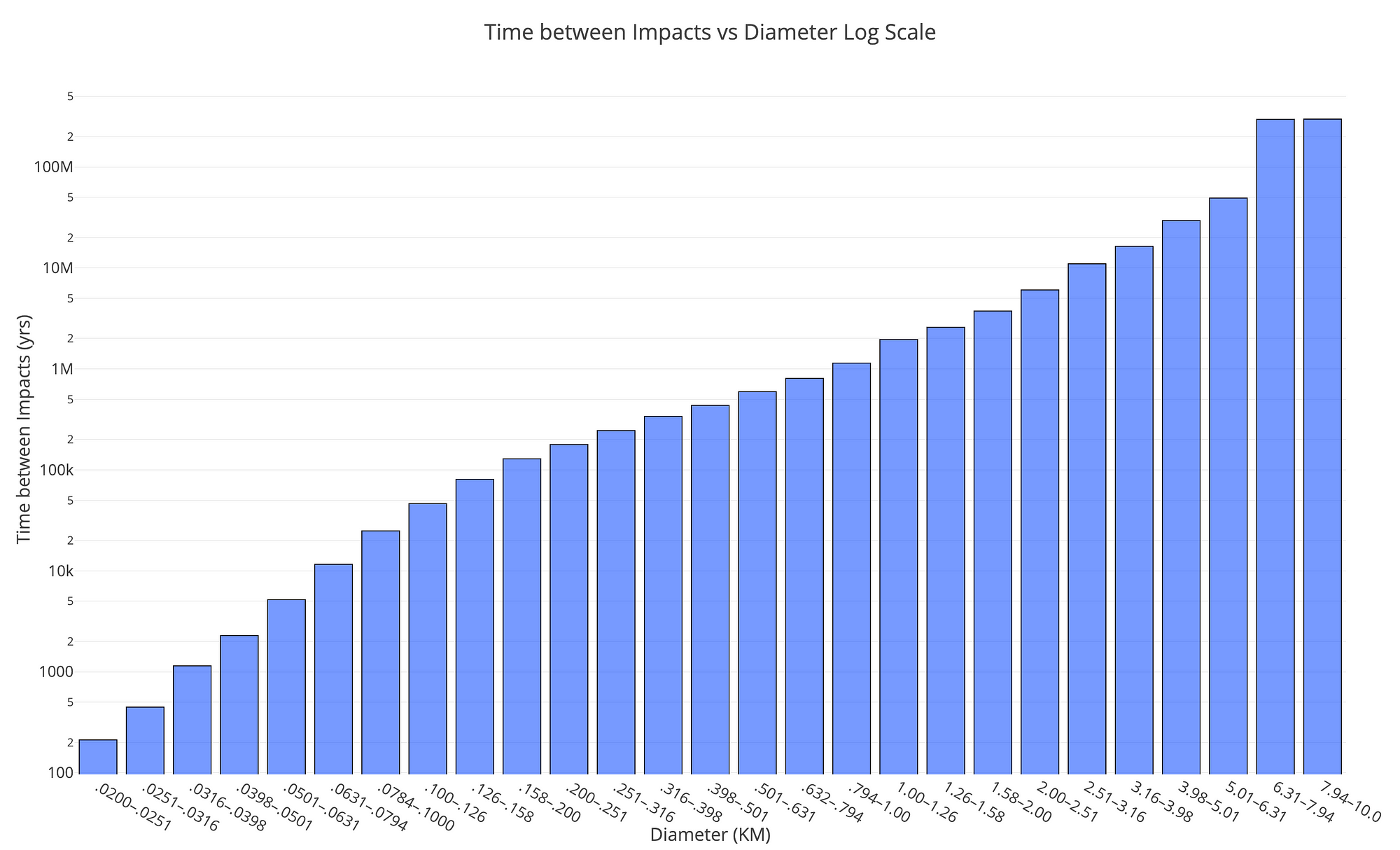
Notice that both graphs are on a log scale and the impact energy is in terms of Megatons Equivalent of TNT. As a point of comparison, the largest human bomb was about 100 Megatons while the largest asteroids are 10 Million Megatons (there are only 2 of these in Earth’s vicinity). From the time between impacts graph, the frequency of impacts decreases rapidly as the size of the asteroids increases to more than 100 million years between impacts.

To explore the data, there’s an interactive exploration tool in the notebook.

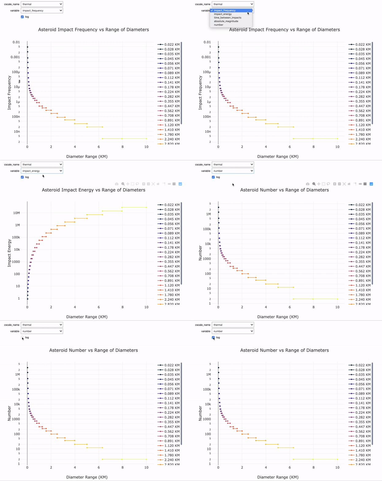Interactive data exploration tool in notebook.

Based on the data exploration, we should expect fewer impacts from the larger asteroids because they have a lower impact frequency. If our modeling results don’t line up with this conclusion, something is probably not right!

Simulating Asterid Impacts

Our objective is to determine the probability distribution of the number of expected impacts in each size category which means we need a time range. To keep things in perspective, we’ll start with 100 years, about the lifespan of a human. This means our distribution will show the probabities for number of impacts over a human life. Because we are using a probabilistic model, we run multiple trials and then derive distributions of outcomes rather than use one number. For a large sample, we’ll simulate one lifetime 10,000 times.

Simulating a Poisson distribution is simple to do in Python using the np.random.poisson function which generates a number of events according to the Poisson distribution with a given rate parameter, lam. To run 10,000 trials, we set that assize. Here is the code for running the simulation with the impact frequency for the smallest asteroid category.

# Simulate 1 lifetime 10,000 times
years = 100
trials = 10_000

# Extract the first frequency and calculate rate parameter
freq = df['impact_frequency'].iloc[0]
lam = freq * years

# Run simulation
impacts = np.random.poisson(lam, size=trials)

The results are best visualized in a histogram:

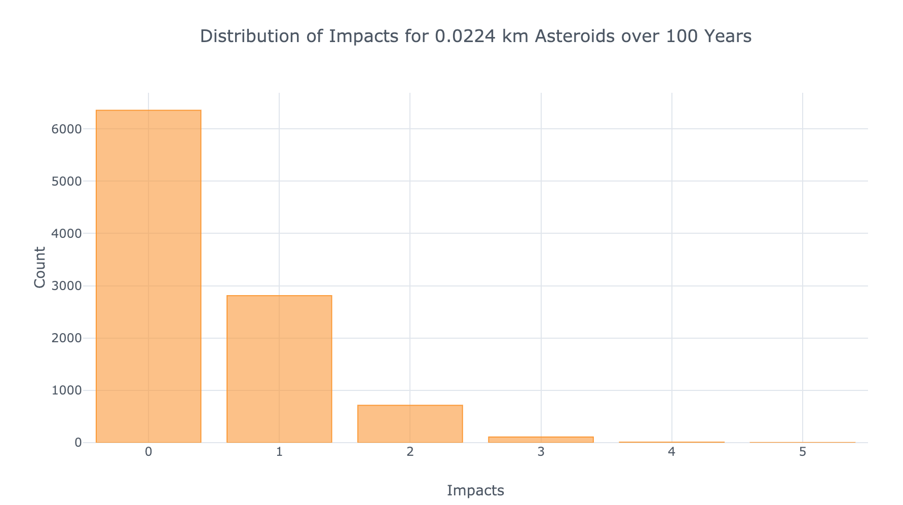Simulation results showing frequency of each number of impacts

We see that over 10,000 simulated lifetimes, the most common number of impacts is 0. This is as expected given the value of the rate parameter (which is the most likely outcome):

print(f'The most likely number of impacts is {lam:.2f}.')

**The most likely number of impacts is 0.47.**

(Since the Poisson Distribution is only defined at discrete number of events, we should round this to the nearest integer).

To compare the simulated results to those expected from theory, we calculate the theoretical probability of each number of impacts using the Poisson Probability Mass Function and the rate parameter:

from scipy.special import factorial

# Possible number of impacts
n_impacts = np.arange(0, 10, 0.25)

# Theoretical probability of each number of impacts
theoretical = np.exp(-lam) * (
               np.power(lam * n_impacts) / factorial(n_impacts))

(We’re using fractional events to get a smooth curve.)

We then plot this on top of the bars (after normalizing to get a probability):

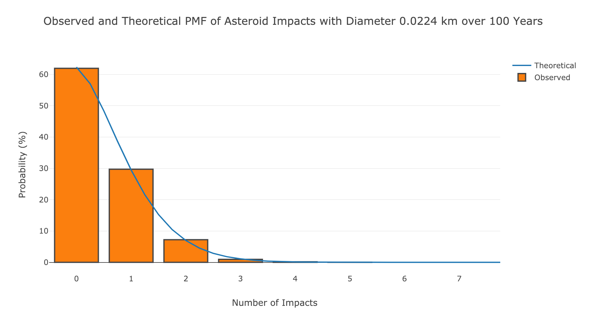Observed and theoretical number of impacts over 100 years for the smallest asteroids.

It’s nice when the observed (in this case simulated) results line up with theory! We can extend our analysis to all sizes of asteroids using the same poisson function and vectorized numpy operations:

# Each trial is a human lifetime
trials = 10000
years = 100

# Use all sizes of asteroids
lambdas = years * df['impact_frequency'].values
impacts = np.random.poisson(lambdas, size=(10000, len(lambdas)))
impacts.shape

**(10000, 27)**

This gives us 10,000 simulations of one lifetime for each of the 27 sizes of asteroids. To visualize this data, we’ll plot the average number of impacts for each size range along with the expected number of impacts (rate parameter).

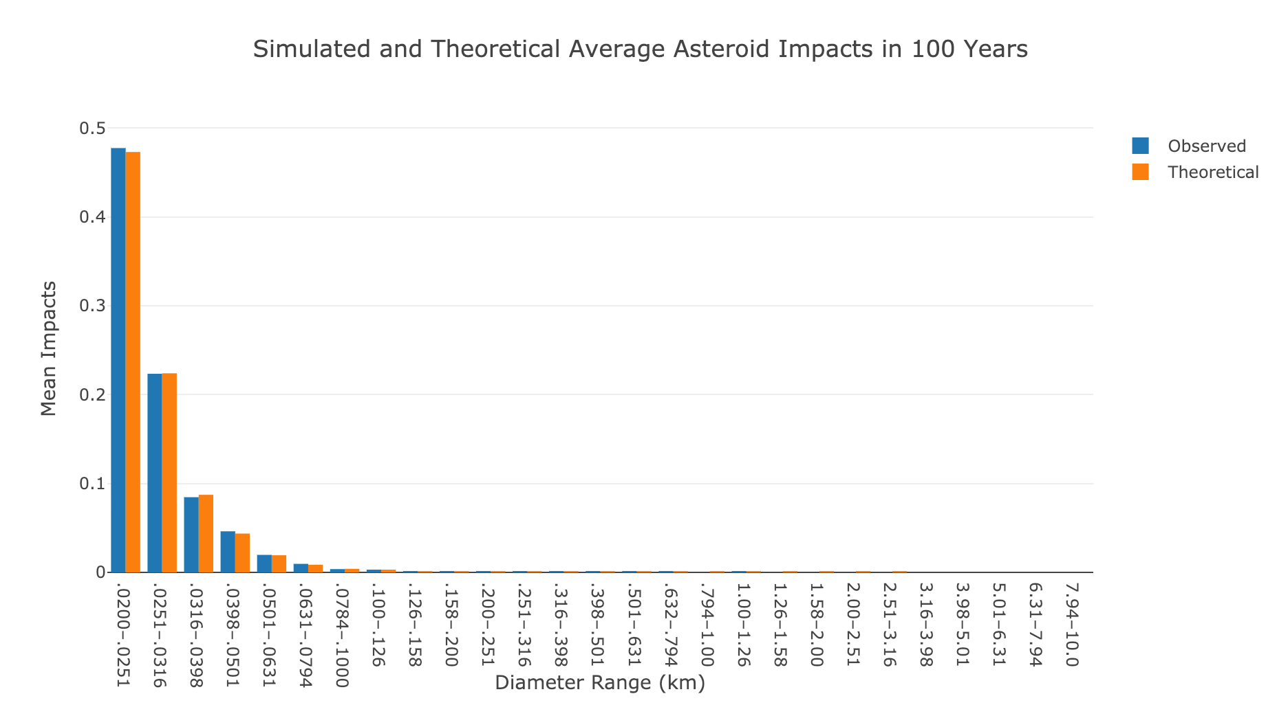Average observed and theoretical number of impacts for all asteroid sizes.

Again, the results line up with theory. For most of the asteroid sizes, there is only a minuscule chance of observing one impact in a lifetime.

For another visualization, we can plot the Poisson PMF for all asteroid sizes:

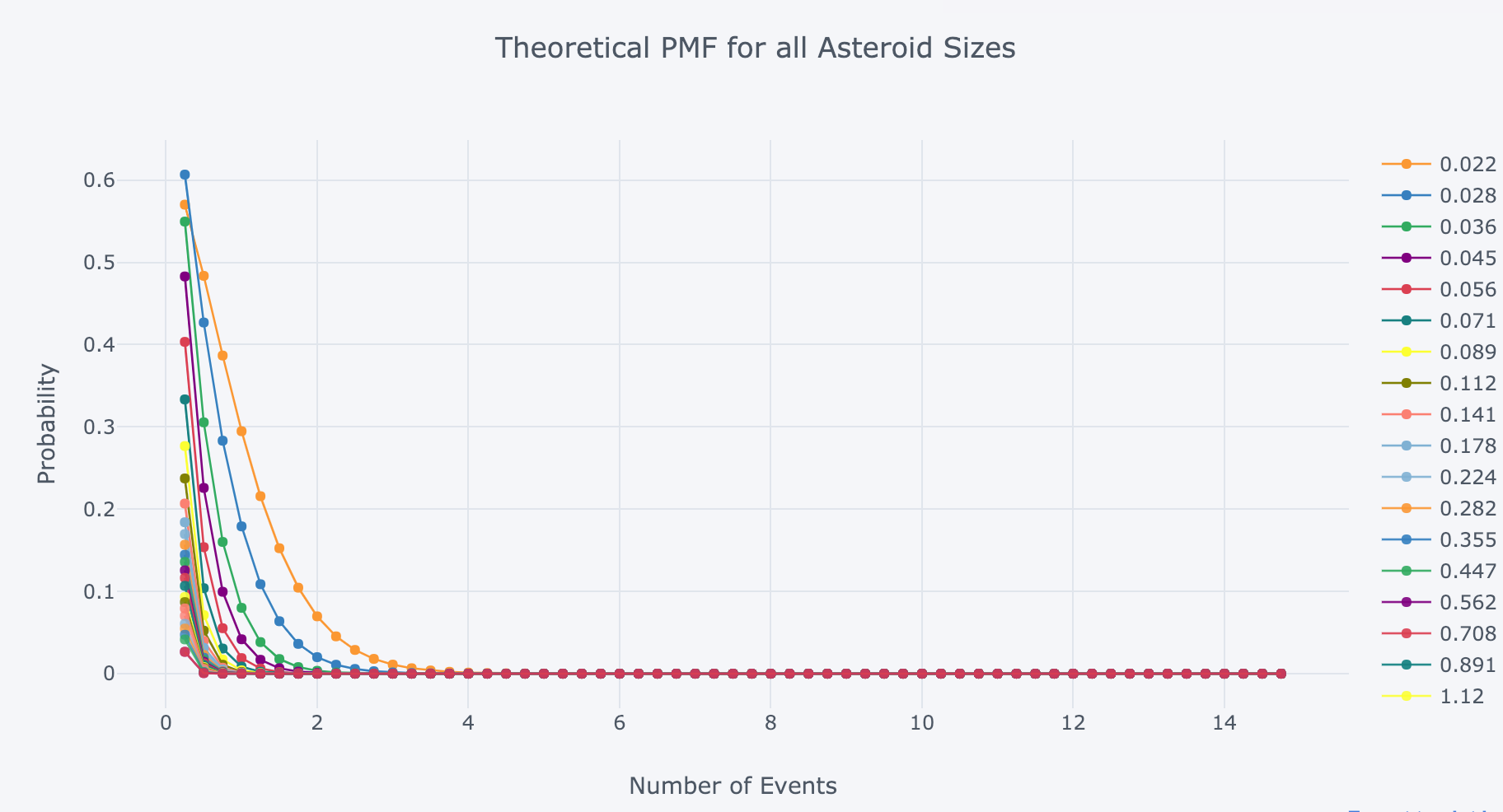Poisson PMF for all asteroids

The most likely number of impacts is 0 for all sizes over 100 years. For those of us alive in 2013, we already had one asteroid event (although not an impact) when a near Earth asteroid 20 m (0.02 km the units used here) in diameter exploded over the Chelyabinsk oblast in Russia. However, because the Poisson process waiting times are memoryless, it is false to conclude there is a lower chance of seeing another asteroid strike now because there was one recently.

Increase the Length of Simulation for more Impacts

In order to see more impacts, we can run the simulation over a longer period of time. Since the genus Homo (our genus) has been around for 2 million years, let’s run 10,000 simulations of 2 million years to see the expected number of asteroid impacts. All we have to do is alter the number of years which in turn affects the rate parameter.

# Simulate 2 million years 10,000 times
years = 2_000_000
trials = 10_000

# Run simulation for all asteroid sizes
lambdas = years * df['impact_frequency'].values
impacts = np.random.poisson(lambdas, size=(10000, len(lambdas)))

Plotting the average number of impacts simulated and theoretical, this time on a log scale, gives us the following:

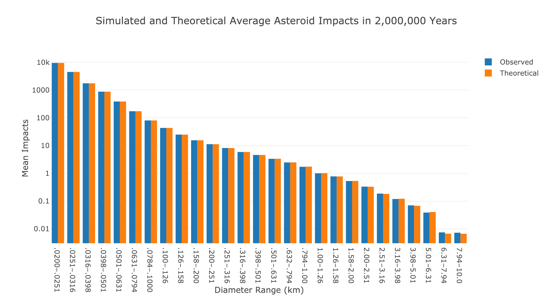Observed and theoretical asteroid impacts over 2 million years.

Now we observe many more impacts which makes sense because we are considering a much longer time period.

The Poisson PMF for all asteroid sizes over 2 million years is:

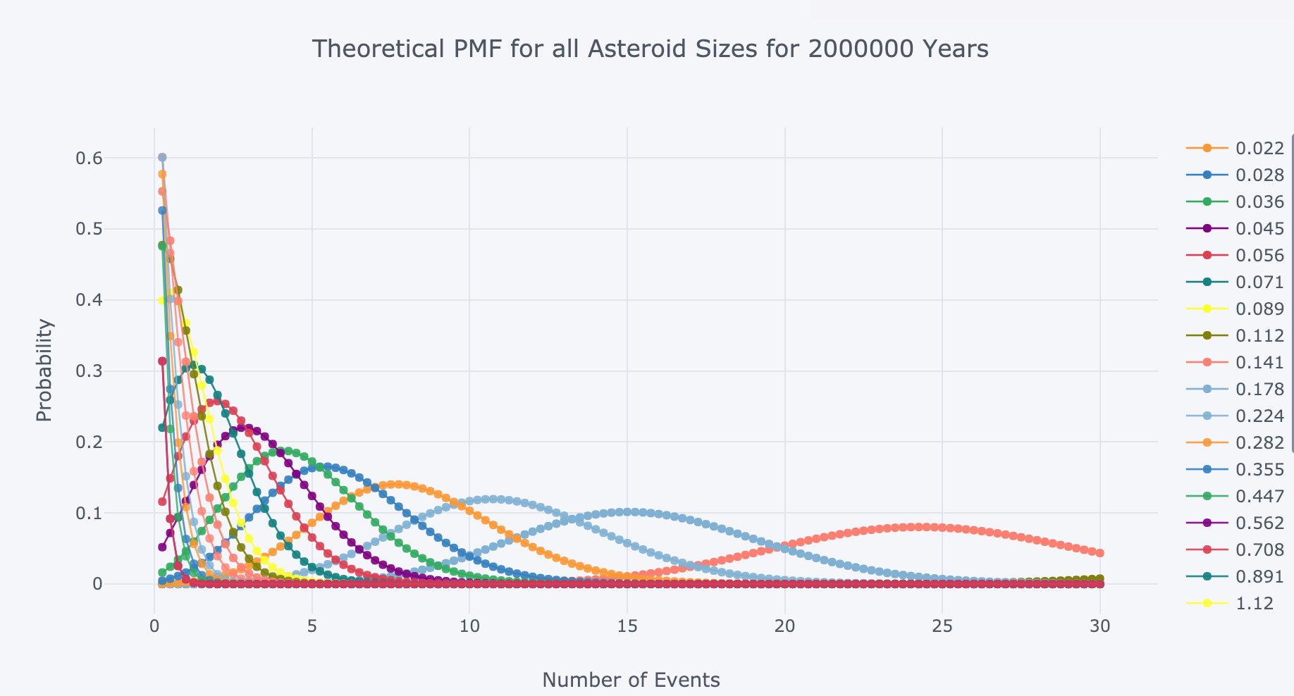Poisson PMF for all asteroid sizes over 2 million years.

Again, the expected (average) number of impacts will be the rate parameter, λ, for each asteroid size.

For the longer simulation, we do observe impacts for the larger asteroid sizes.

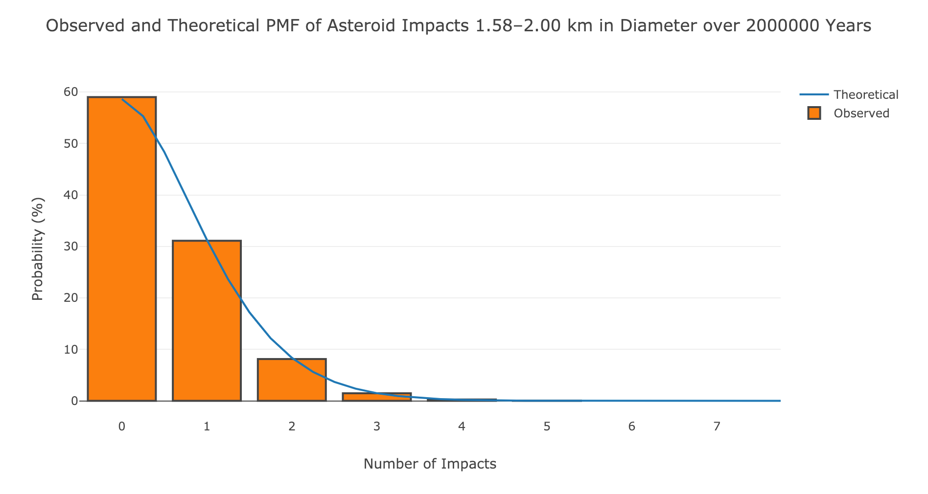Observed and theoretical impacts for larger asteroids over longer time period

Remember, the Chelyabinsk meteor that exploded over Russia was 20 meters in diameter (0.020 km). We are talking some massive asteroids in this graph.

Time Between Impacts

Another way we can use the Poisson Process model is to calculate the time between events. The probability of the time between events exceeding t is given by the following equation:

Calculating the theoretical values is as simple as:

# Frequency for smallest asteroids
freq = df['impact_frequency'].iloc[0]

# Possible waiting times
waiting_times = np.arange(0, 2500)
p_waiting_times = np.exp(-freq * waiting_times)

The relationship follows a decaying exponential:

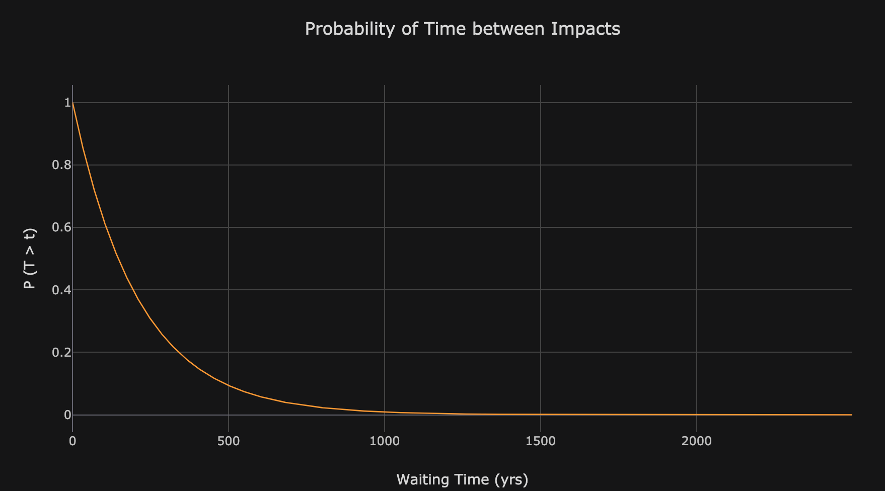Probability distribution for waiting time between asteroid impacts.

To simulate waiting times using the actual data, we can model 100 million years as individual Bernoulli trials (either an impact or not). The probability of success in each year is just the frequency. The waiting time is then the difference in years between impacts (working with the smallest asteroids):

years = 100_000_000

# Simulate Bernoulli trials
impacts = np.random.choice([0, 1], size=years, p=[1-freq, freq])

# Find time between impacts
wait_times = np.diff(np.where(impacts == 1)[0])

Plotting this as a histogram yields the following:

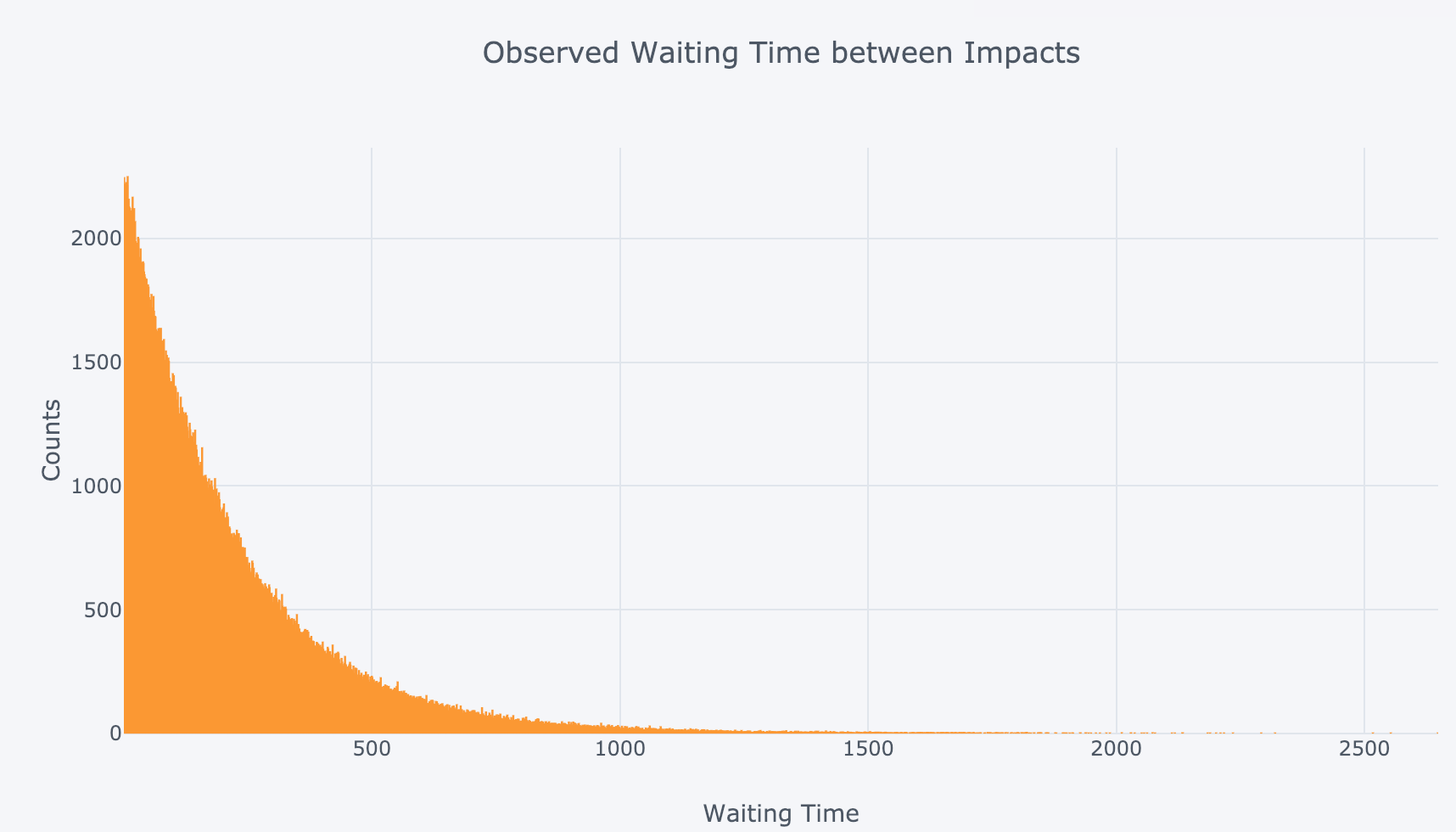Observed waiting time between asteroid impacts for smallest asteroids.

To make sure the observed data lines up with the theoretical, we can plot the two on top of each other (after normalizing and binning):

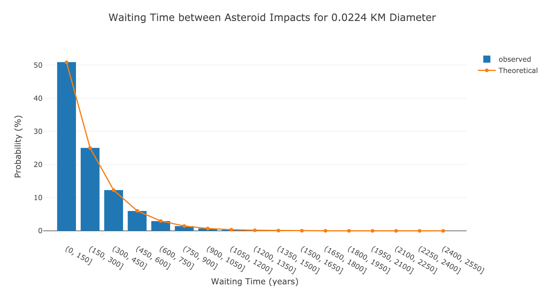Waiting time observed and theoretical for smallest size of asteroids.

As a final plot, we can look at the average time between impacts over all asteroid sizes both observed (simulated) and theoretical:

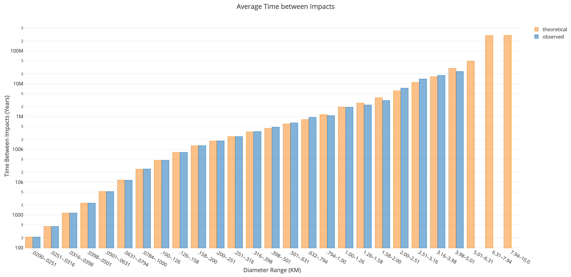Average observed and theoretical waiting time between impacts for all asteroid sizes.

Even over 100 million years, there were no impacts for the largest asteroids (or only one which means we can’t calculate a waiting time). This makes sense because the expected time between impacts is over 100 million years!

Interactive Analysis

The final part in the notebook is an interactive analysis where you can play with the parameters to observe the effects. You can change the length of time to run the simulation, the diameter to inspect, and the number of trials.

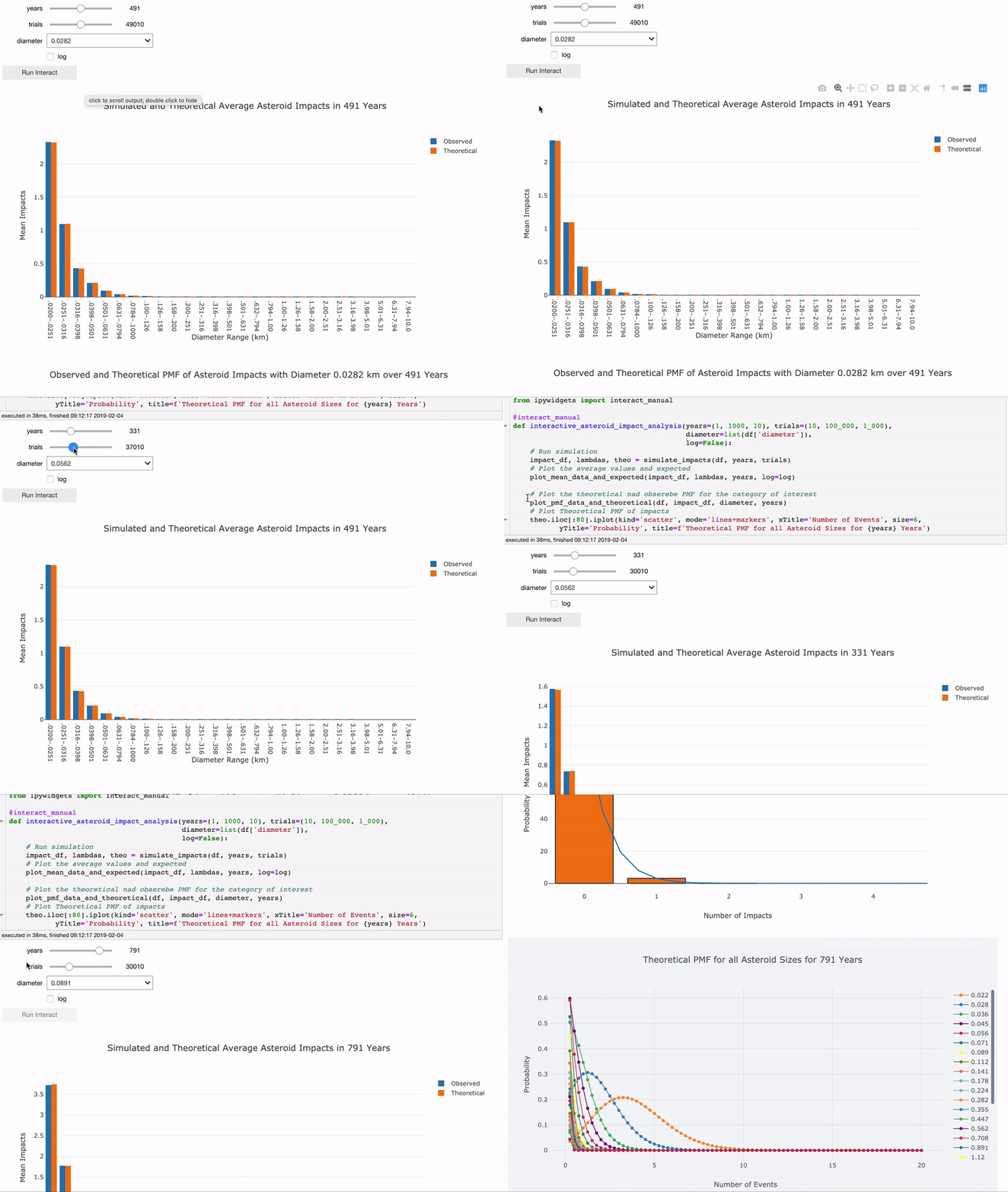Interactive asteroid impacts analysis in Jupyter Notebook.

I encourage you to run the analysis for yourself to see how the parameters change the results by going to the Jupyer Notebook on mybinder.org here.

Conclusions

Many times in school I had the experience of thinking my understanding of a topic was complete in class only to open up the homework and have no idea where to start. This theory-application mismatch was bad enough on the homework and was even larger when it came to real world problems. It wasn’t until my final two years of college when I started learning through doing problems that my ability to apply concepts (and just as importantly my joy in learning) developed. Although the theory is still important (I usually go back to study the concepts after I’ve seen them in use), it can be hard to master a concept only by digging through rigorous derivations.

Any time you encounter a topic you’re having trouble understanding, look for real-world data and start trying to solve problems with the technique. At worst you’ll still be stuck (remember it’s fine to ask for help) but at best you’ll master the method and enjoy the learning process.

In this article, we saw how to apply statistical concepts — the Poisson Process Model and Poisson Distribution — to a real-world situation. Although asteroids probably will not impact our daily lives this project shows a potential use of methods we can apply to other similar problems. Data science requires constantly expanding one’s skill set because of how varied the problems are. Whenever we learn a new technique we become more effective, and if we can enjoy the process by applying a concept to novel data, so much the better.

As always, I welcome feedback and constructive criticism. I can be reached on Twitter @koehrsen_will.