What does it mean to prove something with data?

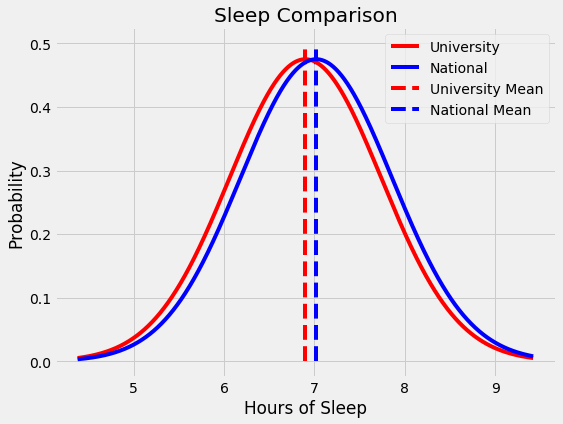
As the dean at a major university, you receive a concerning report showing your students get an average of 6.80 hours of sleep per night compared to the national college average of 7.02 hours. The student body president is worried about the health of students and points to this study as proof that homework must be reduced. The university president on the other hand dismisses the study as nonsense: “Back in my day we got four hours of sleep a night and considered ourselves lucky.” You have to decide if this is a serious issue. Fortunately, you’re well-versed in statistics and finally see a chance to put your education to use!

How can we decide if this is meaningful?

Statistical significance is one of those terms we often hear without really understanding. When someone claims data proves their point, we nod and accept it, assuming statisticians have done complex operations that yielded a result which cannot be questioned. In fact, statistical significance is not a complicated phenomenon requiring years of study to master, but a straightforward idea that everyone can — and should — understand. Like with most technical concepts, statistical significance is built on a few simple ideas: hypothesis testing, the normal distribution, and p values. In this article, we will briefly touch on all of these concepts (with further resources provided) as we work up to solving the conundrum presented above.

Author’s Note: An earlier edition of this post oversimplified the definition of the p-value. I would like to thank Professor Timothy Bates for correcting my mistake. This was a great example of the type of collaborative learning possible online and I encourage any feedback, corrections, or discussion!

The first idea we have to discuss is hypothesis testing, a technique for evaluating a theory using data. The “hypothesis” refers to the researcher’s initial belief about the situation before the study. This initial theory is known as the alternative hypothesis and the opposite is known as the null hypothesis. In our example these are:

• Alternative Hypothesis: The average amount of sleep by students at our university is below the national average for college student.
• Null Hypothesis: The average amount of sleep by students at our university is not below the national average for college students.

Notice how careful we have to be about the wording: we are looking for a very specific effect, which needs to be formalized in the hypotheses so after the fact we cannot claim to have been testing something else! (This is an example of a one-sided hypothesis test because we are concerned with a change in only one direction.) Hypothesis tests are one of the foundations of statistics and are used to assess the results of most studies. These studies can be anything from a medical trial to assess drug effectiveness to an observational study evaluating an exercise plan. What all studies have in common is that they are concerned with making comparisons, either between two groups or between one group and the entire population. In the medical example, we might compare the average time to recover between groups taking two different drugs, or, in our problem as dean, we want to compare sleep between our students and all the students in the country.

The testing part of hypothesis tests allows us to determine which theory, the null or alternative, is better supported by the evidence. There are many hypothesis tests and we will use one called the z-test. However, before we can get to testing our data, we need to talk about two more crucial ideas.

The second building block of statistical significance is the normal distribution, also called the Gaussian or bell curve. The normal distribution is used to represent how data from a process is distributed and is defined by the mean, given the Greek letter μ (mu), and the standard deviation, given the letter σ (sigma). The mean shows the location of the center of the data and the standard deviation is the spread in the data.

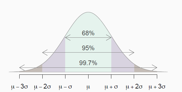Normal Distribution with mean μ and standard deviation σ

The application of the normal distribution comes from assessing data points in terms of the standard deviation. We can determine how anomalous a data point is based on how many standard deviations it is from the mean. The normal distribution has the following helpful properties:

• 68% of data is within ± 1 standard deviations from the mean
• 95% of data is within ± 2 standard deviations from the mean
• 99.7% of data is within ± 3 standard deviations from the mean

If we have a normal distribution for a statistic, we can characterize any point in terms of standard deviations from the mean. For example, average female height in the US is 65 inches (5’ 5”) with a standard deviation of 4 inches. If we meet a new acquaintance who is 73 inches tall, we can say she is two standard deviations above the mean and is in the tallest 2.5% of females. (2.5% of females will be shorter than μ — 2σ (57 in) and 2.5% will be taller than μ+2σ).

In statistics, instead of saying our data is two standard deviations from the mean, we assess it in terms of a z-score, which just represents the number of standard deviations a point is from the mean. Conversion to a z-score is done by subtracting the mean of the distribution from the data point and dividing by the standard deviation. In the height example, you can check that our friend would have a z-score of 2. If we do this to all the data points the new distribution is called the standard normal with a mean of 0 and a standard deviation of 1 as shown below.

Transformation from normal (right) to standard normal distribution (left). (Source)

Every time we do a hypothesis test, we need to assume a distribution for the test statistic, which in our case is the average (mean) hours of sleep for our students. For a z-test, the normal curve is used as an approximation for the distribution of the test statistic. Generally, according to the central limit theorem, as we take more averages from a data distribution, the averages will tend towards a normal distribution. However, this will always be an estimate because real-world data never perfectly follows a normal distribution. Assuming a normal distribution lets us determine how meaningful the result we observe in a study is. The higher or lower the z-score, the more unlikely the result is to happen by chance and the more likely the result is meaningful. To quantify just how meaningful the results are, we use one more concept.

The final core idea is that of p-values. A p-value is the probability of observing results at least as extreme as those measured when the null hypothesis is true. That might seem a little convoluted, so let’s look at an example.

Say we are measuring average IQ in the US states of Florida and Washington. Our null hypothesis is that average IQs in Washington are not higher than average IQs in Florida. We perform the study and find IQs in Washington are higher by 2.2 points with a p-value of 0.346. This means, in a world where the null hypothesis — average IQs in Washington are not higher than average IQs in Florida — is true, there is a 34.6% chance we would measure IQs at least 2.2 points higher in Washington. So, if IQs in Washington are not actually higher, we would still measure they are higher by at least 2.2 points about 1/3 of the time due to random noise. Subsequently, the lower the p-value, the more meaningful the result because it is less likely to be caused by noise.

Whether or not the result can be called statistically significant depends on the p-value (known as alpha) we establish for significance _before_we begin the experiment . If the observed p-value is less than alpha, then the results are statistically significant. We need to choose alpha before the experiment because if we waited until after, we could just select a number that proves our results are significant no matter what the data shows!

Choosing a p-value after the study in one good way to “Lie with Statistics”

The choice of alpha depends on the situation and the field of study, but the most commonly used value is 0.05, corresponding to a 5% chance the results occurred at random. In my lab, I see values from 0.1 to 0.001 commonly in use. As an extreme example, the physicists who discovered the Higgs Boson particle used a p-value of 0.0000003, or a 1 in 3.5 million chance the discovery occurred because of noise. (Statisticians are loathe to admit that a p-value of 0.05 is arbitrary. R.A. Fischer, the father of modern statistics, choose a p-value of 0.05 for indeterminate reasons and it stuck)!

To get from a z-score on the normal distribution to a p-value, we can use a table or statistical software like R. The result will show us the probability of a z-score lower than the calculated value. For example, with a z-score of 2, the p-value is 0.977, which means there is only a 2.3% probability we observe a z-score higher than 2 at random.

The percentage of the distribution below a z-score of 2 is 97.7%

As a summary so far, we have covered three ideas:

1. Hypothesis Testing: A technique used to test a theory
2. Normal Distribution: An approximate representation of the data in a hypothesis test.
3. p-value: The probability a result at least as extreme at that observed would have occurred if the null hypothesis is true.

Now, let’s put the pieces together in our example. Here are the basics:

• Students across the country average 7.02 hours of sleep per night according to the National Sleep Foundation
• In a poll of 202 students at our university the average hours of sleep per night was 6.90 hours with a standard deviation of 0.84 hours.
• Our alternative hypothesis is the average sleep of students at our university is below the national average for college students.
• We will use an alpha value of 0.05 which means the results are significant f the p-value is below 0.05.

First, we need to convert our measurement into a z-score, or the number of standard deviations it is away from the mean. We do this by subtracting the population mean (the national average) from our measured value and dividing by the standard deviation over the square root of the number of samples. (As the number of samples increases, the standard deviation and hence the variation decreases. We account for this by dividing the standard deviation by the square root of the number of samples.)

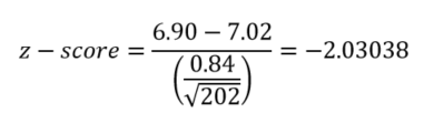Conversion to z-score

The z-score is called our test-statistic. Once we have a test-statistic, we can use a table or a programming language such as R to calculate the p-value. I use code here not to intimidate but to show how easy it is to implement our solution with free tools! (# are comments and bold is output)

# Calculate the results
z_score = (6.90 - 7.02) / (0.84 / sqrt(202))
p_value = pnorm(z_score)

# Print our results
sprintf('The p-value is %0:5f for a z-score of %0.5f.', p_value, z_score)

**"The p-value is 0.02116 for a z-score of -2.03038."**

Based on the p-value of 0.02116, we can reject the null hypothesis. (Statisticians like us to say reject the null rather than accept the alternative.) There is statistically significant evidence our students get less sleep on average than college students in the US at a significance level of 0.05. The p-value shows there is a 2.12% chance that our results occurred because of random noise. In this battle of the presidents, the student was right.

Before we ban all homework, we need to be careful not to assign too much to this result. Notice that our p-value, 0.02116, would not be significant if we had used a threshold of 0.01. Someone who wants to prove the opposite point in our study can simply manipulate the p-value. Anytime we examine a study, we should think about the p-value and the sample size in addition to the conclusion. With a relatively small sample size of 202, our study might have statistical significance, but that does mean it is practically meaningful. Further, this was an observational study, which means there is only evidence for correlation and not causation. We showed there is a correlation between students at our school and less average sleep, but not that going to our school causes a decrease in sleep. There could be other factors at play that affect sleep and only a randomized controlled study is able to prove causation.

As with most technical concepts, statistical significance is not that complex and is just a combination of many small ideas. Most of the trouble comes with learning the vocabulary! Once you put the pieces together, you can start applying these statistical concepts. As you learn the basics of stats, you become better prepared to view studies and the news with a healthy skepticism. You can see what the data actually says rather than what someone tells you it means. The best tactic against dishonest politicians and corporations is a skeptical, well-educated public!

As always, I welcome constructive criticism and feedback. I can be reached on Twitter @koehrsen_will.