How to avoid being fooled by randomness

The CEO of a major drug company has a problem. The new miracle drug developed by his chemists to do increase willpower has failed in every trial. The CEO cannot believe these results, but the researchers tell him there is no evidence of an effect on willpower at a significance level (p-value) of 0.05. Convinced the drug must be beneficial in some way, the CEO has a brilliant idea: instead of testing the drug for just one effect, test it for 1000 different effects at the same time, all at the same p-value. Even if it doesn’t increase willpower, it must do something, like reduce anxiety or boost memory. Skeptical, the researchers redo the trials exactly as the CEO says, monitoring 1000 different health measures of subjects on the drug. The researchers come back with astounding news: the drug had a significant effect on 50 of the measured values! Miraculous right? Actually, it would be more surprising if they had found no significant effects with this experimental analysis.

The CEO’s mistake is an example of the multiple comparisons problem. The issue comes down to the noisiness of data in the real world. While the chance of noise affecting one result may be small, the more measurements we make, the larger the probability that a random fluctuation is mis-classified as a meaningful result. While this affects researchers performing objective studies, it can also be used for nefarious purposes.

The CEO has a drug that he wants to sell but it doesn’t do what it was designed for. Instead of admitting failure, he instructs his researchers to keep looking until they find some vital sign the drug improves. Even if the drug has absolutely no effect on any health markers, the researchers will eventually find it does improve some measures because of random noise in the data. For this reason, the multiple comparisons problem is also called the look-elsewhere effect: if a researcher doesn’t find the result she wants, she can just keep looking until she finds some beneficial effect!

If at first you don’t succeed, just keep searching!

Fortunately, most statisticians and researchers are honest and use methods to account for the multiple comparisons problem. The most common technique is called the Bonferroni Correction, but before we can explain it, we need to talk about p-values.

The p-value represents the probability that in a world where the null hypothesis is true, the test statistic would be at least as extreme as the measured value. In the drug example, for the initial trial, the null hypothesis is that the drug does not increase the average motivation of individuals. The alternative hypothesis, or the researcher’s belief, is the drug increases average motivation. With a p-value of 0.05, this means in a world where the drug does not increase average motivation, the researchers would measure the drug does increase motivation 5% of the time due to random noise.

Before a study is run, researchers select a p-value (known as alpha or the significance level) for establishing statistical significance. If the measured p-value falls below the the threshold, the null hypothesis is rejected and the results are statistically significant. A lower measured p-value is considered better because it shows the results are less likely to occur by chance.

Once we know what a p-value represents, we can spot the CEO’s mistake. He ordered the trial to be run again with the same p-value of 0.05, but instead of testing for just one effect, he wanted to test for 1000. If we perform 1000 hypothesis tests with a p-value of 0.05, we would expect on average to find 50 significant results due to random noise (5% of 1000). Some of the results might actually be meaningful, but it would be unethical to declare they all are and sell the drug based on this study!

The figure below illustrates the issue. I generated 1000 random numbers from a standard normal distribution and plotted them on the corresponding probability density function. We can ignore the y-axis here and focus on the x-axis which is in terms of the z-score. If we perform a hypothesis test and assume the mean of our test statistic (measured value) comes from a normal distribution, then we calculate our test-statistic in terms of a z-score. Using our selected p-value (alpha) for the hypothesis test, we can then find the z-score needed for statistical significance. These thresholds for a p-value of 0.05 are shown as the red vertical lines, with observations outside the lines considered to be statistically significant. The black dots are insignificant randomly generated observations, while the red dots are “significant” randomly generated data points.

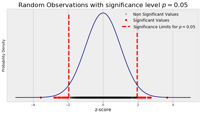Random Observations with a p value of 0.05

We can see with random observations and using an uncorrected p-value, we classify a number of these results as significant! This might be great news if we have a drug to sell, but as responsible data scientists, we need to account for performing multiple tests so we are not misled by noise.

A simple fix to the multiple comparisons problem is the Bonferroni Correction. To compensate for many hypothesis tests, we take the p-value for a single comparison and divide it by the number of tests. In the case of the drug company trial, the original p-value of 0.05 should be divided by 1000, resulting in a new significance threshold of 0.00005. This means results must be more extreme for them to be considered significant, decreasing the probability that random noise is characterized as meaningful.

We can apply the Bonferroni Correction to the graph made above and see how it affects the classification of random points. The graph has the same structure, but now the significance thresholds account for multiple tests.

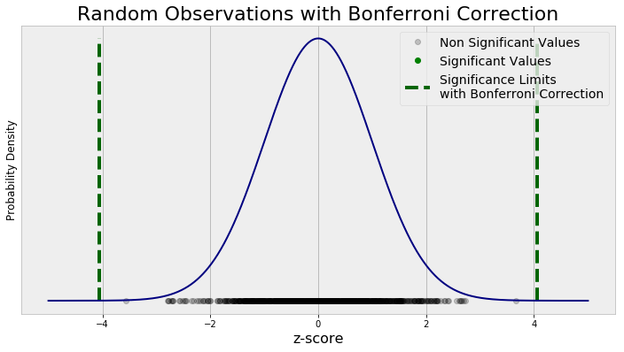Random Observations with Bonferroni Correction to Significance Level

No random data points are now considered significant! There are criticisms that the Bonferroni Correction is too conservative and it may lead us to reject some results which actually are meaningful. However, the important concept behind the method is the significance value needs to be adjusted when we make many comparisons.

The problem of multiple comparisons extends to more than just hypothesis tests. If we compare enough data sets, we can find correlations that are nothing more than random noise. This is humorously illustrated by the website Spurious Correlations which has examples of completely unrelated trends that happen to closely follow each other.

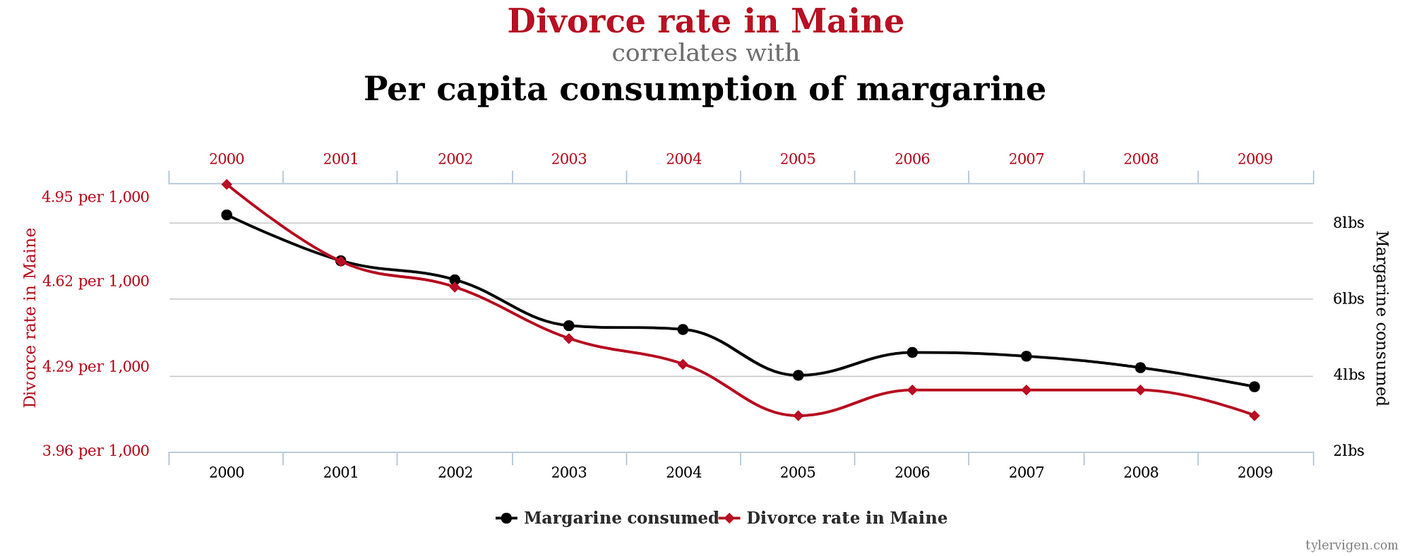Seems Legit (Source)

The multiple comparisons issue is important to keep in mind when we examine studies, but it can also be used in our daily lives. If we look hard enough, we can find correlations anywhere, but that does not mean we should make lifestyle changes because of them. Maybe we weigh ourselves every day and find our weight is negatively correlated with the number of text messages we send. It would be foolish to send more text messages in the hopes of losing weight. Humans are adept at spotting patterns, and when we look hard enough and make enough comparisons, we can convince ourselves there is meaning in random noise. Once we are aware of this tendency, we are prepared to analyze dubious claims and make rational choices.

As always, I welcome feedback and constructive criticism. I can be reached on Twitter @koehrsen_will.