How to quickly create a powerful exploratory data analysis visualization

Once you’ve got yourself a nice cleaned dataset, the next step is Exploratory Data Analysis (EDA). EDA is the process of figuring out what the data can tell us and we use EDA to find patterns, relationships, or anomalies to inform our subsequent analysis. While there are an almost overwhelming number of methods to use in EDA, one of the most effective starting tools is the pairs plot (also called a scatterplot matrix). A pairs plot allows us to see both distribution of single variables and relationships between two variables. Pair plots are a great method to identify trends for follow-up analysis and, fortunately, are easily implemented in Python!

In this article we will walk through getting up and running with pairs plots in Python using the seaborn visualization library. We will see how to create a default pairs plot for a rapid examination of our data and how to customize the visualization for deeper insights. The code for this project is available as a Jupyter Notebook on GitHub. We will explore a real-world dataset, comprised of country-level socioeconomic data collected by GapMinder.

Pairs Plots in Seaborn

To get started we need to know what data we have. We can load in the socioeconomic data as a pandas dataframe and look at the columns:

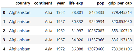Each row of the data represents an observation for one country in one year and the columns hold the variables (data in this format is known as tidy data). There are 2 categorical columns (country and continent) and 4 numerical columns. The columns are fairly self-explanatory: life_exp is life expectancy at birth in years, popis population, and gdp_per_cap is gross domestic product per person in units of international dollars.

The default pairs plot in seaborn only plots numerical columns although later we will use the categorical variables for coloring. Creating the default pairs plot is simple: we load in the seaborn library and call the pairplot function, passing it our dataframe:

# Seaborn visualization library
import seaborn as sns

# Create the default pairplot
sns.pairplot(df)

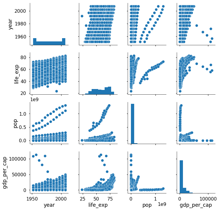I’m still amazed that one simple line of code gives us this entire plot! The pairs plot builds on two basic figures, the histogram and the scatter plot. The histogram on the diagonal allows us to see the distribution of a single variable while the scatter plots on the upper and lower triangles show the relationship (or lack thereof) between two variables. For example, the left-most plot in the second row shows the scatter plot of life_exp versus year.

The default pairs plot by itself often gives us valuable insights. We see that life expectancy and gdp per capita are positively correlated showing that people in higher income countries tend to live longer (although this of course does not prove that one causes the other). It also appears that (thankfully) life expectancies worldwide are on the rise over time. From the histograms, we learn that the population and gdp variables are heavily right-skewed. To better show these variables in future plots, we can transform these columns by taking the logarithm of the values:

# Take the log of population and gdp_per_capita
df['log_pop'] = np.log10(df['pop'])
df['log_gdp_per_cap'] = np.log10(df['gdp_per_cap'])

# Drop the non-transformed columns
df = df.drop(columns = ['pop', 'gdp_per_cap'])

While this plot alone can be useful in an analysis, we can find make it more valuable by coloring the figures based on a categorical variable such as continent. This is also extremely simple in seaborn! All we need to do is use the hue keyword in the sns.pairplot function call:

sns.pairplot(df, hue = 'continent')

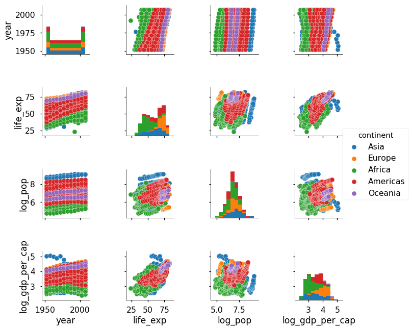Now we see that Oceania and Europe tend to have the highest life expectancies and Asia has the largest population. Notice that our log transformation of the population and gdp made these variables normally distributed which gives a more thorough representation of the values.

This graph is more informative, but there are still some issues: I tend not to find stacked histograms, as on the diagonals, to be very interpretable. A better method for showing univariate (single variable) distributions from multiple categories is the density plot. We can exchange the histogram for a density plot in the function call. While we are at it, we will pass in some keywords to the scatter plots to change the transparency, size, and edgecolor of the points.

# Create a pair plot colored by continent with a density plot of the # diagonal and format the scatter plots.

sns.pairplot(df, hue = 'continent', diag_kind = 'kde',
             plot_kws = {'alpha': 0.6, 's': 80, 'edgecolor': 'k'},
             size = 4)

The density plots on the diagonal make it easier to compare distributions between the continents than stacked bars. Changing the transparency of the scatter plots increases readability because there is considerable overlap (known as overplotting) on these figures.

As a final example of the default pairplot, let’s reduce the clutter by plotting only the years after 2000. We will still color by continent, but now we won’t plot the year column. To limit the columns plotted, we pass in a list of vars to the function. To clarify the plot, we can also add a title.

# Plot colored by continent for years 2000-2007
sns.pairplot(df[df['year'] >= 2000],
             vars = ['life_exp', 'log_pop', 'log_gdp_per_cap'],
             hue = 'continent', diag_kind = 'kde',
             plot_kws = {'alpha': 0.6, 's': 80, 'edgecolor': 'k'},
             size = 4);

# Title
plt.suptitle('Pair Plot of Socioeconomic Data for 2000-2007',
             size = 28);

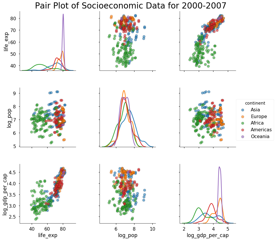This is starting to look pretty nice! If we were going to do modeling, we could use information from these plots to inform our choices. For example, we know that log_gdp_per_cap is positively correlated with life_exp, so we could create a linear model to quantify this relationship. For this post we’ll stick to plotting, and, if we want to explore our data even more, we can customize the pairplots using the PairGrid class.

Customization with PairGrid

In contrast to the sns.pairplot function, sns.PairGrid is a class which means that it does not automatically fill in the plots for us. Instead, we create a class instance and then we map specific functions to the different sections of the grid. To create a PairGrid instance with our data, we use the following code which also limits the variables we will show:

# Create an instance of the PairGrid class.
grid = sns.PairGrid(data= df_log[df_log['year'] == 2007],
                    vars = ['life_exp', 'log_pop',
                    'log_gdp_per_cap'], size = 4)

If we were to display this, we would get a blank graph because we have not mapped any functions to the grid sections. There are three grid sections to fill in for a PairGrid: the upper triangle, lower triangle, and the diagonal. To map plots to these sections, we use the grid.map method on the section. For example, to map a scatter plot to the upper triangle we use:

# Map a scatter plot to the upper triangle
grid = grid.map_upper(plt.scatter, color = 'darkred')

The map_upper method takes in any function that accepts two arrays of variables (such as plt.scatter)and associated keywords (such as color). The map_lower method is the exact same but fills in the lower triangle of the grid. The map_diag is slightly different because it takes in a function that accepts a single array (remember the diagonal shows only one variable). An example is plt.hist which we use to fill in the diagonal section below:

# Map a histogram to the diagonal
grid = grid.map_diag(plt.hist, bins = 10, color = 'darkred',
                     edgecolor = 'k')

# Map a density plot to the lower triangle
grid = grid.map_lower(sns.kdeplot, cmap = 'Reds')

In this case, we are using a kernel density estimate in 2-D (a density plot) on the lower triangle. Put together, this code gives us the following plot:

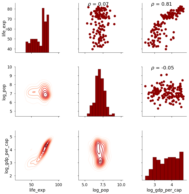
The real benefits of using the PairGrid class come when we want to create custom functions to map different information onto the plot. For example, I might want to add the Pearson Correlation Coefficient between two variables onto the scatterplot. To do so, I would write a function that takes in two arrays, calculates the statistic, and then draws it on the graph. The following code shows how this is done (credit to this Stack Overflow answer):

Our new function is mapped to the upper triangle because we need two arrays to calculate a correlation coefficient (notice also that we can map multiple functions to grid sections). This produces the following plot:

The correlation coefficient now appears above the scatterplot. This is a relatively straightforward example, but we can use PairGrid to map any function we want onto the plot. We can add as much information as needed provided we can figure out how to write the function! As a final example, here is a plot that shows the summary statistics on the diagonal instead of a plot.

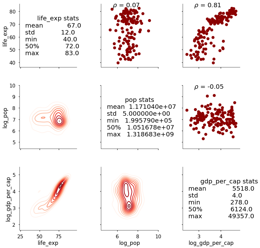This needs a little cleaning up, but it shows the general idea; in addition to using any existing function in a library such as matplotlib to map data onto the figure, we can write our own function to show custom information.

Conclusion

Pairs plots are a powerful tool to quickly explore distributions and relationships in a dataset. Seaborn provides a simple default method for making pair plots that can be customized and extended through the Pair Grid class. In a data analysis project, a major portion of the value often comes not in the flashy machine learning, but in the straightforward visualization of data. A pairs plot is provides us with a comprehensive first look at our data and is a great starting point in data analysis projects.

I welcome feedback and constructive criticism and can be reached on Twitter @koehrsen_will.