Udacity Machine Learning Engineer Nanodegree Capstone Project

Author’s Note: This is the report I completed for my Udacity Machine Learning Engineer Nanodegree Capstone Project. All work is original and feel to use/expand upon/disseminate. [Numbers in brackets are citations to the sources listed in the references section].

I. Definition

Project Overview

Safety and reliability testing is a crucial step in the automobile manufacturing process. Every new vehicle design must pass a thorough evaluation before it enters the consumer market. Testing can be time-consuming and cost-intensive as a full check of vehicle systems requires subjecting the car to all situations it will encounter in its intended use. Predicting the overall time for a vehicle to pass testing is difficult because each model requires a different test stand configuration.[1] Mercedes-Benz has been a pioneer of numerous vehicle safety and technology features and offers a range of custom options for each model. Every possible vehicle combination must undergo the same rigorous testing to ensure the vehicle is robust enough to keep occupants safe and withstand the rigors of daily use. The large array of options offered by Mercedes means a large number of tests for the company’s engineers to conduct. More tests result in more time spent on the test stand, increasing costs for Mercedes and generating carbon dioxide, a polluting greenhouse gas. Efforts by Mercedes Benz and other automakers to improve the efficiency of vehicle testing procedures have mainly focusing on developing automated test systems.[2][3] An automatic test system eliminates the variability inherent in human behavior, is safer than allowing humans in the driver’s seat, and results in an overall more efficient evaluation process.

The Mercedes-Benz “Greener Manufacturing” Competition hosted by Kaggle[1] pursues a related approach to optimizing the vehicle testing process by encouraging the development of a machine learning model that is able to predict the testing duration based on a particular vehicle combination. The stated goal of the competition is to reduce the time vehicles spend on the test stand which consequently will decrease carbon dioxide emissions associated with the testing procedure. Although the reduction in carbon dioxide may not be noteworthy on a global scale,4 improvements to Mercedes’s process can be passed along to other automakers or even to other industries which could result in a significant decrease in carbon dioxide emissions. Moreover, one of the fundamental tenets of machine learning is that the efficiency of current systems can be improved through the use of the massive quantities of data now routinely collected by companies. Kaggle is a website dedicated to that proposition where companies create machine learning competitions with a stated objective and provide the public a dataset to apply to the problem. Competitions such as those offered on Kaggle, or the X-Prizes,[5] have been demonstrated to spur innovation [6] and help attract individuals and teams looking to hone their skills, participate in cutting-edge challenges, and perhaps win a modest prize. For this project, I created a model to participate in the Greener Manufacturing competition. All required data for the Greener Manufacturing competition was provided by Mercedes-Benz. The dataset was collected from thousands of safety and reliability tests run on a variety of Mercedes vehicles.

Problem Statement

The objective of the Mercedes-Benz Greener Manufacturing competition is to develop a machine learning model that can accurately predict the time a car will spend on the test bench based on the vehicle configuration. The vehicle configuration is defined as the set of customization options and features selected for the particular vehicle. The motivation behind the problem is that an accurate model will be able to reduce the total time spent testing vehicles by allowing cars with similar testing configurations to be run successively. This problem is an example of a machine learning regression task because it requires predicting a continuous target variable (the duration of the test) based on one or more explanatory variables [7] (the configuration of the vehicle). This problem is also a supervised task because the targets for the training data are known ahead of time and the model will learn based on labeled data. The steps to solving the problem are as follows:

1. Download the Mercedes vehicle testing data from Kaggle.

2. Prepare the data to feed into the machine learning model.

3. Select an appropriate algorithm/method for the problem.

4. Optimize the model using the labeled training data.

5. Make predictions on the unlabeled testing data and submit to the competition.

6. Iterate on 3–5 to improve the model to an acceptable standard.

Mercedes-Benz will implement the best-performing model into the vehicle design and manufacturing process to increase the overall efficiency of the testing procedure while maintaining high safety and reliability standards.

Metrics

The evaluation metric for the competition is the R^2 measure, known as the coefficient of determination. R^2 is a measure of the quality of a model that is used to predict one continuous variable from a number of other variables. [8] It describes the amount of variation in the dependent variable, in this case the testing time of a vehicle in seconds, based on the independent variables, in this case the combination of vehicle custom features, that can be explained by the model. It is often interpreted as the percentage of the variation in the targets that is explained by the features. Thus, an R^2 value of 0.6 indicates that 60% of the variation in the testing time could be explained by the variation in the vehicle set-up. The remaining 40% of the variance is either not captured by the model, or is due to lurking variables that have not been included in the data. The coefficient of determination is expressed mathematically [9] as

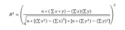Equation 1: Coefficient of Determination

where n is the number of instances (vehicle tests), x is the prediction for the instance (the predicted test time in seconds), and y is the known truth value for the instance (the known testing time in seconds). An R^2 of 0 can be achieved by simply drawing a straight line through the data at the mean value of the target variable. The best possible coefficient of determination value is 1.0 which would indicate that the model explains all the of the variance in the response variable in terms of the input variables.

The coefficient of determination is the appropriate metric for the problem because the goal, as defined by Mercedes-Benz, is to create a model that is able to determine the testing time of a vehicle. Mercedes is interested in why different vehicles take different times to test and how this can be represented in a machine learning model. Therefore, the algorithm that best explains the variation in testing times will be the optimal machine learning model for the task. Moreover, the evaluation metric used to determine the winner of the competition is the coefficient of determination. The coefficient of determination is a common metric used in regression tasks and is implemented in Scikit-Learn, where it is the default evaluation score for a regressor.10 The coefficient of determination for the training data can be ascertained during the model evaluation phase because the training data includes the known target values; however, R^2 for the testing data can only be found by submitting the predictions from the model to the competition. Five predictions are allowed per participant per day, which limits the amount of possible evaluation on the test set.

II. Analysis

Data Exploration

Two data files are provided by Mercedes-Benz for use in the competition: a training dataset, and a testing dataset. Both files are provided in the comma separated value (CSV) format and are available for download on the Kaggle competition data page. [11] The training and testing data both contain 4209 vehicle tests obtained by Mercedes for a range of vehicle configurations. The training data also contains the target variable, or testing duration in seconds, for each vehicle test. No target is provided for the testing data as the testing durations are known only by Mercedes and are used to determine the winner of the competition. Each vehicle test is defined by the vehicle configuration, which is encoded in a set of features. Both the training and the testing dataset contain 376 different vehicle features with names such as ‘X0’, ‘X1’, ‘X2’ and so on. All of the features have been anonymized meaning that they do not come with a physical representation. The description of the data does indicate that the vehicle features are configuration options such as suspension setting, adaptive cruise control, all-wheel drive, and a number of different options that together define a car model. There are 8 categorical features, with values encoded as strings such as ‘a’, ‘b’, ‘c’, etc. The other 368 features are binary, meaning they either have a value of 1 or 0. Each vehicle test has also been assigned an ID which was not treated as a feature for this analysis. An image of a representative subset of the training data is shown below:

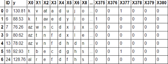Figure 1: Training Data Sample

A brief summary table of the testing and training dataset follows:

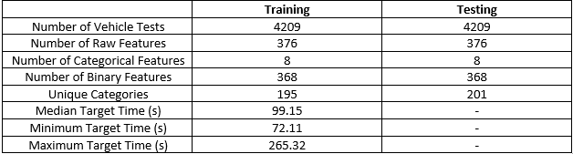Table 1: Training and Testing Dataset Characteristics

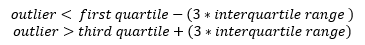
Although the data has been cleaned by Mercedes prior to being made available for the competition and therefore there are no errors or missing entries, the data may still contain outliers with respect to vehicle testing time. These outliers could be valid data but are extreme enough to affect the performance of the model. The definition of a strong outlier is expressed mathematically [12] as:

Equation 2: Defition of Strong Outlier

where the first quartile is the value that 25% of the numbers fall beneath, the third quartile is the value that 75% of the numbers fall beneath, and the interquartile range (IQR) is the different between the third and first quartile. Given this definition of an outlier, there were 4 vehicle tests that classified as extreme on the upper end of the vehicle testing time. The Exploratory Visualization section further examines the outliers within the dataset.

In order for the machine learning model to process the categorical variables, they must be one-hot encoded. [7] This means that the unique categories contained in the categorical variable are transformed into a set of new variables. Each instance is assigned a one for the new variable corresponding to its original categorical variable and a zero in all other new variables. This is best illustrated by Figure 2.

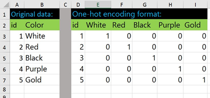Figure 2: One-Hot Encoding [13]

One-hot encoding transform all of the features to binary values. After both the testing and training data had been one-hot encoded, the two datasets were aligned in order to eliminate any features that were present in one dataset but not in the other. This is necessary because the model would not know how to respond it if encountered a feature in the testing set that it had not seen in the training data. After one-hot encoding and alignment of the training and testing data there were a total of 553 binary features in both datasets.

Exploratory Visualization

The first aspect of the data to investigate was the target variable, the vehicle testing duration. The plot below shows all of the testing times arranged from shortest to longest from left to right. The four outliers can be seen at right with the highest value shown in red. Plotting the data demonstrates the extreme nature of this data point more effectively than examining the numbers.

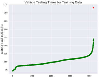Figure 3: Vehicle Testing Times for Training Data

The testing times can also be visualized as a histogram. For this visualization, the outlying data point has been removed in order to better represent the majority of the data.

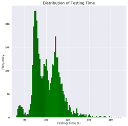Figure 4: Testing Times for Training Data Histogram

There are several conclusions to be drawn from this histogram:

· The majority of test durations are between 90 and 100 seconds

· There are peaks in testing times around 97–98 seconds and near 108 seconds.

· The testing times are bi-modal, with two distinct peaks.

· This data is positively skewed, with a long tail stretching into the upper values. [14]

Based on the target variable visualization, I concluded that I was justified in removing one outlier, the training data point with the greatest testing time. Although it is a valid data point, it is extreme enough that it will adversely affect the performance of the algorithm (as shown in the Evaluation section).

The second half of the data exploration phase focused on the vehicle features. I began with the categorical variables by plotting the testing durations versus the unique category in boxplots. [8] This was done for each of the categorical variables on the training data.

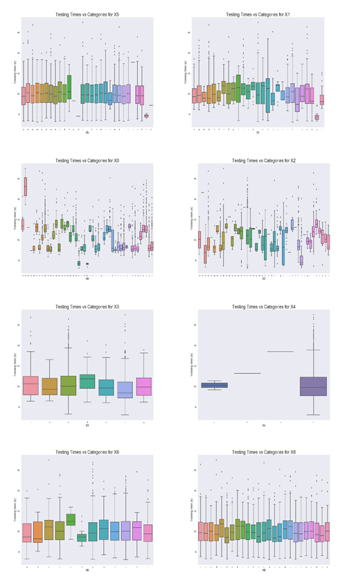Figure 5: Categorical Variable Boxplots

There are no discernible trends within the categorical variables with respect to vehicle testing duration. Moreover, it is difficult to draw intuitive conclusions from this exercise because the features have no physical representation. Further exploration of the binary features also proved inconclusive. The plot below shows the distribution of the binary features in both the training and testing set. The zeros, indicating that the car did not have the feature, are shown in orange, and the ones, representing that the car had the option, are shown in blue.

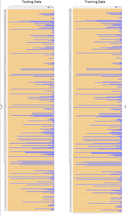Figure 6: Distribution of Binary Variables

With this particular problem, it was difficult to draw any conclusions from the visualizations of the explanatory variables. Figure 6 demonstrates that some of the binary features are shared by all of the vehicles and some are shared by none. Looking further into the numerical data for the testing set, I identified 12 binary variables where the values were either all 1 or 0. As there is no variation in these features, they have no predictive power and therefore, these 12 features may be removed. The data exploration has underscored the need for dimensionality reduction. Fortunately, one common technique for reducing the number of features, Principal Components Analysis (PCA), is an unsupervised technique that does not require an understanding of the physical representation of the features. [7] PCA played a crucial role in reducing the input number of features into the algorithm and as discussed in the Data Preprocessing section. The conclusions from the data exploration are as follows:

· One outlier, as determined by vehicle testing duration, needs to be removed

· 12 binary variables encode no information and should be removed

· There are no noticeable trends within the categorical or binary variables

· Unsupervised dimensionality reduction (PCA) will need to be performed on the data

Algorithms/Techniques

The final model created for this project combines a number of different machine learning techniques. At the highest level, the final model is a weighted vote between two intermediate models. The first intermediate model is an ensemble method known as extreme gradient boosting [15] that works by building numerous simple regressors on top of each other to create a final strong regressor. The second intermediate model is a stacked model in which another ensemble method, an extra trees forest [16], builds on top of a regularized linear regression. The architecture is shown below in Figure 7.

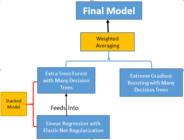Figure 7: Architecture of Complete Model

The final model was derived based upon research from books, the Kaggle discussion forum, and papers discussing the benefits and drawbacks of various models. Nearly all of the top-performing models in the Kaggle competition used the XGBoost method averaged with or stacked on top of other ensemble methods. This is where I derived the top level architecture. From that point, it was a matter of determining which models best complimented one another. Based on the benchmark model, I saw that a Linear Regression performed quite well, but tended to overfit the training data. Therefore, my stacked model incorporated a Linear Regression with regularization to reduce the amount of overfitting. The choice of an Extra Trees forest was made by determining the performance of ensemble methods stacked on top of the Linear Regression. Based on the individual performance of each intermediate model, it was evident that combining the two predictions in a weighted average would help to improve the robustness of the model. The full process for designing the algorithms and optimizing them for the problem is discussed in the Implementation section.

To explain how the model functions, it is best to start at the lowest level, the linear regression with elastic net regularization. The full workings of a linear regression are explained in the Benchmark Model section, and elastic net is one of many methods to regularize a linear model. Regularization can be thought of as constraining a model’s complexity in order to prevent overfitting on the training data. [7] Overfitting means that the model “memorizes” the training data leading to poor generalization on new instances the model has not seen before. A model that overfits the training data is said to have high variance and low bias. Regularization can reduce the variance of a model by reducing the degrees of freedom within the model and can be performed on a linear model by reducing the magnitude of the model parameters. Elastic Net regularization applies a penalty to each model parameter in the cost function which encourages the model to select smaller parameters during training. [7] Elastic Net is one of a number of regularization functions which differ in the type of penalty applied during training.

The idea of a stacked model [17] is relatively simple: the outputs (predictions) of the first model are used as inputs into the second model. In this case, during training, the predictions (vehicle testing durations) from the Linear Regression with regularization are fed as inputs into the Extra Trees Forest regressor along with the known target labels. The Extra Trees regressor thus learns to make predictions based on the prediction from the previous model and the known true values. The Extra Trees regressor is what is known as an ensemble method. [7] It works by combining multiple simpler models into one complex model, thereby reducing the variance from a single model and generating better predictions. The Extra Trees regressor is built of many individual Decision Tree algorithms. A Decision Tree creates a flowchart (tree)of questions (generally in the form of thresholds for the features) during training to split the data points into ever smaller bins, each with a different predicted target value. During testing, the Decision Tree moves through the flowchart one node at a time and places the data point in the appropriate bin based on the features of the instance. A simple model of a decision tree is presented below.

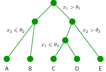Figure 8: Decision Tree Model [18]

In this case, the x terms would be features, the θ terms would be thresholds established during training, and the letters would be the final predicted target. An Extra Trees regressor trains many decision trees and takes a vote of all the trees to determine the final prediction for each instance.

The stacked model forms one half of the final model. The other half is composed of another ensemble method, called Extreme Gradient Boosting. The principal behind extreme gradient boosting is the same as that of the Extra Trees regressor except in this case, the individual decision trees are trained sequentially and each tree is trained on the previous tree’s residuals, or the difference between the tree’s prediction and the true value.

Equation 3: Residual

By training on the residuals, or errors in the predictions, each successive tree becomes better at predicting the most difficult to predict instances (those with the largest residuals) and over time, the ensemble becomes more powerful than a single classifier. The final prediction is a weighted average over all of the individual predictions, with the more confident trees receiving a higher weighting. Gradient boosting has become one of the algorithms of choice for machine learning competitions because of its predictive power. Decision trees form the basis for both ensemble methods because they are relatively quick to train and have well-established default parameters.

At the top level, the final model takes an average of the predictions from each intermediate model. The weighting given to each model can be determined through an iterative process of adjusting the weighting and determining the model’s performance. During training, the preprocessed data will be passed to both intermediate models. The Extreme Gradient model will learn the thresholds for each leaf in the forest of decision trees it trains. The stacked model will first pass the training data through the linear regression, where the model will learn the parameters (weighting) to apply to each feature, then the linear regression will make a prediction for each training point and pass that on as input to the Extra Trees Forest along with the known target values. The Extra Trees regressor will likewise form its own forest of decision trees with the thresholds for each split determined during training. When testing, each new instance will be passed to both intermediate models. In the case of the stacked model, a prediction will be made by the linear regression and then the Extra Trees Regressor will make a prediction based on the output from the linear regression. The Gradient Boosting model will generate its own prediction. The overall prediction will then be an average from the two intermediate models. The architecture of the model is relatively complex, but the fierce (yet friendly) competition on Kaggle encourages the development of unique models in order to achieve slight performance increases.

Benchmark Model

A benchmark model for this regression task is a linear regression. Linear regression is a method for modeling the relationship between a target variable (also called the response variable) and one or more independent, explanatory variables. [7] When there are more than one explanatory variables, this process is called multiple linear regression. In this situation, the target variable is the testing time of the car and the explanatory variables are the customization options for the car. A linear regression model assumes that the response variable can be represented as a linear combination of the model parameters (coefficients) and the explanatory variables. The benchmark model in this situation is a basic linear regression that predicts the target for an instance based on the instance’s features multiplied by the model’s parameters (coefficients) and added to a bias term. This is shown as an equation below:

Equation 4: Linear Regression Model

where y is the target (predicted) variable, the c terms are the model parameters (coefficients) and the x terms are the feature values. When the model trains, it learns the set of parameters, and when it is asked to make a prediction, it takes the instance’s feature values and multiplies by the parameters to generate a prediction. The default method for Linear Regression in Scikit-learn is ordinary least squares, where the model calculates parameters that minimize the sum of the squared difference between the prediction and the known targets. [19]

Initially, I used the entire set of raw features for creating a benchmark model. However, this resulted in a negative coefficient of determination, indicating that the model was performing worse than if it had drawn a constant line at the mean of the data. To develop a more reasonable benchmark, I decided to reduce the dimensionality of the data. I found the Pearson’s Correlation Coefficient, or R, between all of the individual features and the target variable. The correlation coefficient describes the strength and direction of the linear relationship between an independent and dependent variable. [20] A value of 1.0 would indicate a perfectly linear positive relationship and thus the Pearson coefficient can be used as one method to determine which features will be useful when predicting a target variable. Once I had identified the correlation coefficients, I trained a number of linear regressors using a range of the most positively correlated features. The top-scoring model used the 47 top correlated features. I selected this as the benchmark model because of the reasonable R^2 value which would take some effort to better. The final benchmark model scored a 0.56232 coefficient of determination on the testing set using five-fold cross validation (cross validation is discussed in the Implementation section). The predictions made on the testing set scored a 0.54549 coefficient of determination when submitted into the Kaggle competition. As of June 25, this score was only good enough for 2400 on the competition leaderboard [21] out of roughly 3000 competitors.

The benchmark serves as a comparison for the final model. In order to declare the project a success, the final model will need to significantly outperform the benchmark model on the R^2 measure. The final model should score higher both on the training dataset, using five-fold cross validation, and on the testing set, when the predictions are submitted to the competition.

III. Methodology

Data Preprocessing

There are several interrelated steps in the data preprocessing workflow [7]:

· Obtaining and cleaning data

· Data preparation

· Feature engineering/ Dimensionality reduction

The first step requires obtaining the data in a usable format. For this project, no “data wrangling” was required because the data was already provided in an organized format on the Kaggle competition page. Data preparation mainly consisted of one-hot encoding the categorical variables, removing the outliers, and removing features that do not encode any information. In the training data, there was a single outlier with a testing time far greater than that of the next highest value. This point was removed so that it would not skew the predictions of the regression. There were also 12 binary features with values that were either all 1’s or 0’s. These variables (they cannot even be called variables because they do not change, but should be referred to as constants) do not contain any information and were removed. After aligning the training and testing datasets to ensure they contained the same number of features, I was left with a training set of 4208 data points with labels and 531 features. The testing set has 4209 data points and 531 features without labels.

The final step in the data preprocessing pipeline is feature engineering. This encompasses a range of operations including adding new features or removing features to reduce the dimensionality of the data. Based on the data exploration, I decided that I would not be able to create brand new features by combining existing features because I did not observe any trends within the variables. Therefore, I concentrated on reducing the number of features. One implementation of this is documented in the Benchmark Model section where I used a subset of features selected by ranking the variables in terms of correlation coefficient with respect to the target variable. Another method involves selecting the most relevant features for a given algorithm. Within Scikit-learn, there are a number of algorithms that will display the feature importances after training. Both of the ensemble methods explored in this report have a feature importances attribute. [22] However, I received substantially different results when comparing the weights given to each feature for both models. Consequently, I decided that selecting a smaller number of features based on feature importances was not the correct decision.

After some experimentation, the dimensionality reduction method that I did implement is an unsupervised technique known as Principal Components Analysis (PCA). [23] PCA creates a set of basis vectors that represent the dimensions along which the original data has the greatest variation. In other words, the original data is projected onto a new axis with the greatest variance in order to reduce the dimensions while preserving the maximum amount of information. The first principal component explains the greatest variance in the data, while the second explains the second most and is orthogonal to the first and so on. A common technique is to keep the number of principal components that explain a given percentage of the variance within a dataset. After some trial and error, I decided to retain the Principal Components that explained 95% of the variation in the data. The meant keeping the first 140 principal components as can be seen in the graph below:

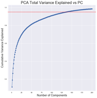Figure 9: PCA Total Variance Explained vs. Number of Principal Components

The 140 principal components selected explain 95.31% of the variance in the data. The PCA algorithm was trained on the training features and then the training features are transformed by projecting the original features along the first 140 principal components. The testing data features are transformed by the already-trained PCA model. Applying PCA considerably reduces the number of dimensions within the data and should lead to improved performance by reducing the noise in the data.

Implementation

All of the code for this project was written in Python 2.7 and executed in an interactive Jupyter Notebook. The main Python library used for the project was Scikit-learn, a popular machine learning framework. Although the dataset is not large by machine learning standards, training the various models and performing hyperparameter optimization on my personal laptop in a timely manner was not feasible. Therefore, I ran the Jupyter Notebook on a Google Cloud server.

The development of the final regression model can be split into two sections.

I. Model Selection

II. Hyperparameter tuning (discussed in the Refinement section)

The first stage involved testing and evaluating a selection of algorithms. Different algorithms are suited for different tasks, and the best way to determine the correct algorithm is to try them out on the dataset. I began this process as usual by referring to the Scikit-learn algorithm selection flowchart. The relevant section of the chart for choosing a regression algorithm is shown below.

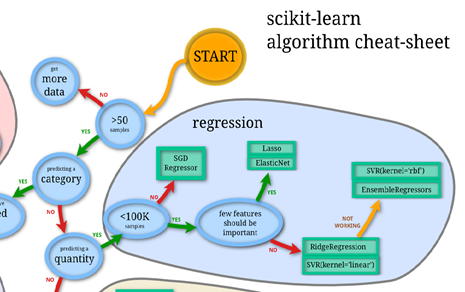Figure 10: Scikit-learn Model Selection for Regression Tasks [24]

As this was a regression task with fewer than 100,000 samples (training data points), there were several starting options. My approach was to evaluate a number of the simple algorithms recommended, and if none were sufficient, I would proceed to ensemble methods. The results of evaluating a number of simple classifiers are shown below. As is demonstrated in the table, the only simple model that outperformed the benchmark was the Support Vector regressor with an rbf kernel. All of the simple models were evaluated with the 140 principal components from the data preprocessing and were created with minimal hyperparameter tuning. The objective at this stage was simply to evaluate the models to determine if any were acceptable for the problem. I expected that I would have to move on to ensemble methods, but in some machine learning tasks, a simple model is able to capture all of the relationships within the data and can perform very well.

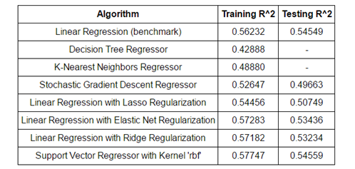Table 2: Summary of Model Performance

Examining the performance of the simple regressors, it was clear I would have to employ a more sophisticated model to significantly improve on the benchmark. The next logical place to turn, as evidenced by the flowchart and on the discussion boards for the Kaggle Competition, [25] was ensemble methods. Ensemble methods work to create a model by combining multiple or building upon many simple models. [26] There are two commonly identified classes of ensemble methods:

· Bagging

· Boosting

Bagging [27] (short for bootstrap aggregating) uses the “wisdom” of the crowd to create a better model than an individual regressor. If training a single model is like asking one business analyst to make a prediction given an entire dataset, bagging is like taking the average forecast of an entire roomful of analysts, each of whom have seen a small part of the data. For example, an Extra Trees regressor trains numerous Decision Trees, with each tree fit on a different subset of the data. In the bagging technique, these subsets are randomly chosen, and the final prediction is attained by averaging all of the predictions. The implementation used in this project set the Bootstrap parameter to false meaning that the subsets are not replaced after being used for training, a technique known as pasting [28]). Boosting is based on a similar idea, except each successive simple model is trained on the most “difficult” subset of the data. The first model is trained on the data, and then the data points with predictions that are the furthest away from the true values (as determined by the residuals, or the difference between the prediction and the known target value) are used to trained the second model and so on. Over time, the entire ensemble will become stronger by concentrating on the hardest to learn data. The final prediction is a weighted average of all the individual regressors with the most “confident” trees given the highest weighting. One boosting technique that is very popular for machine learning competitions is known as XGBoost, [29] which stands for extreme gradient boosting. Both of the ensemble methods used in this project are based on many individual Decision Trees. Decision Trees are a popular choice to use in an ensemble because of their well-established default hyperparameters and relatively rapid training time. Studies [26][30] have shown ensemble methods are more accurate than a single classifier because they reduce the variance that can arise in a single classifier. Bagging was observed to almost always have better performance than a single model, and boosting generally performed better depending on the dataset and the model hyperparameters.

The final model used both an Extra Trees and an Extreme Gradient Boosting ensemble method in Scikit-learn. [31] The Extra Trees algorithm was part of a stacked model built on top of a Linear Regression with Elastic Net Regularization. There were three major problems that I encountered while developing the model:

· Algorithm training and predicting time

· Diminishing returns to algorithm optimization

· Limited number of testing opportunities

The first problem arose when I was running Grid Search to determine the best parameters for the algorithms. Many of the parameter grids contained over 100 models to test, and because I was using five-fold cross-validation, the total time to carry out the Grid Search was a significant obstacle. I soon realized I would have to invest time into learning how to use cloud-based computing services. I was successfully able to figure out how to run a Jupyter Notebook on a Google Cloud server, and I am sure that this skill will be invaluable moving forward as the size of datasets and the complexity of algorithms continue to increase and deep learning becomes commonplace in machine learning implementations.

Implementing basic algorithms in Scikit-learn is relatively simple because of the high level of abstraction within the library. The actual theory behind the algorithms is hidden in favor of usability. Moreover, the default parameters are given reasonable values to allow a user to have a usable model up and running quickly. [32] In this project, I found it relatively simple to get the baseline model functioning with a decent coefficient of determination. However, as in most machine learning projects, the law of diminishing returns soon crept in with regards to hyperparameter tuning. [33] Improving the performance of any model even a few tenths of a percentage point required a significant time investment in tuning the algorithm. The full effect of these diminishing returns can be seen in the complexity of the final model. As the development of the model progressed, it became difficult to determine what steps to take to improve the performance. Mostly, I tried to combat this by using Grid Search to find the optimal parameters. This problem was an example of the effectiveness of data, [34] a phenomenon where the quality and preprocessing of the training data has much greater importance to the final model performance than the tuning of the algorithm.

Finally, the structure of the Kaggle competition allowed for minimal evaluation on the testing set. The Kaggle competition is set up to only allow users to make five submissions per twenty-four hours. This meant that it was difficult to compare the relative performance of models as they were developed on the testing set. I repeatedly would test the algorithms using five-fold cross validation on the training set, but these results were not always in alignment with performance on the testing set when I would make my submissions. The models routinely scored lowered on the testing set than on the training set as expected, but there was not always a correlation between R^2 on the training and on the testing set. For example, some intermediate models scored a higher coefficient of regression on the training set but then scored lower on the testing set. The main way that I overcame this problem was by testing as much as possible on the training set using cross-validation, and then making submissions only on the models in which I had the most confidence.

Refinement

Once the structure of the final algorithm had been selected, the next step was to optimize the model. This mainly consisted of what is known as hyperparameter tuning. (The word ‘hyperparameter’ refers to an aspect of the algorithm set by the programmer before training, such as the number of trees in a Random Forest, or the number of neighbors to use in a Nearest Neighbors implementation. The word ‘parameters’ refers to the learned attributes of the model, such as the coefficients in a linear regression).7 I like to think of this step as adjusting the settings of the model to optimize them for the problem. This can be done manually, by changing one or more hyperparameters at a time and then checking the model performance. However, a more efficient method for parameter optimization is to perform a grid search. There are two primary aspects to this method in Scikit-learn with the GridSearchCV class:

· Hyperparameter search

· Cross validation

The idea of grid search is to define a set of hyperparameters, known as a grid, and then allow an algorithm to test all of the possible combinations. Most of the default hyperparameters in Scikit-learn are reasonable, and my methodology when performing a grid search was therefore to try values for parameters both above and below the default value. Depending on which configuration returned the best score, I would then perform another search with the hyperparameters moving in the direction that increased scores. The CV in GridSearchCV stands for cross validation, which is a method to prevent overfitting on the training data. The concept behind cross-validation is that the data is first split into a training and testing set. Then, the training data is split into ’n’ smaller subsets, known as folds. Each iteration through the cross validation, the algorithm is trained on n-1 on these subsets and evaluated on the nth subset. The final score of the algorithm is the average score across all of the folds. This prevents overfitting whereby the model learns the training data very well, but then cannot generalize to new data that it has not seen before. After n iterations of cross-validation have been completed, the model is evaluated one final time on the test set to determine the performance on a previously unseen set of data. Cross-validation is combined with Grid Search to optimize the algorithm for the given problem while also ensuring that the variance of the model is not too high so that the model can generalize to new instances. GridSearchCV allows a wide range of models to be evaluated more efficiently than manually checking each option.

The final hyperparameters for the constituent models that make up the final model are presented in Table 3. Any hyperparameters not specified in the table were set to the default value in Scikit-learn.

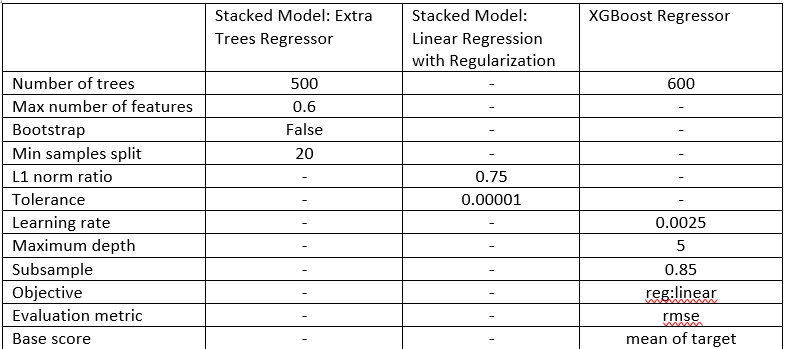Table 3: Model Hyperparameters

GridSearchCV was performed on both intermediate models (the XGBoost model and the stacked model of an Extra Trees regressor stacked on a regularized Linear Regression) individually. The main hyperparameters adjusted for the XGBoost model were the number of decision trees used, the maximum depth of each tree, and the learning rate. The number of trees is simply the number of trees built by the algorithm; the maximum depth of each tree controls the number of levels in each tree and can be used to reduce overfitting or increase the complexity to better learn the relationships within the data; and the learning rate is used in gradient descent to determine how large a step the algorithm takes at each iteration. Compared to the defaults, the learning rate was decreased, the maximum depth of each tree was decreased, and the number of trees was increased. The main parameters adjusted for the other intermediate model were the l1 ratio and tolerance for the Linear Regression and the maximum features, minimum number of samples per leaf, and the number of estimators for the Extra Trees Regressor. The l1 ratio for Elastic Net controls the penalty assigned to the model parameters (it specifies the blend between Ridge and Lasso Regression) and the tolerance is a minimum step size for the algorithm to continue running. In terms of the Extra Trees regressor, the maximum features is the number of features each tree considers, the minimum number of samples per leaf is the minimum number of data points that must be in each leaf node, and the number of estimators is the number of decision trees in the forest. The l1_ratio was increased for Elastic Net which has the effect of increasing the penalty (if the ratio is 1.0, then Elastic Net is equivalent to Lasso Regression which tends to eliminate the least important features by setting the weights close to zero). The maximum number of features for the Extra Trees Regressor was decreased which means that the model did not need to use all the features. Both of these adjustments suggest to me that 140 principal components may have been too many because both models performed implicit feature selection through the hyperparameters. However, keeping too many principal components and then having some not used by the model is preferable to not having enough features and therefore discarding useful information.

The final and most critical hyperparameter was the weighting for the averaging between the two intermediate models. I determined that the best method was to try a range of ratios and submit the resulting predictions to the competition. The final model placed more weight on the XGBoost predictions. However, increasing the contribution from the XGBoost regressor reached a point of diminishing returns above 0.75. Averaging the predictions from the XGBoost model and the stacked model resulted in a significant improvement in the coefficient of determination compared to each model individually as discussed in the next section.

IV. Results

Model Evaluation and Validation

The final model was optimized through a combination of Grid Search with cross validation and manually adjusting the final weighting attributed to each of the intermediate models. The Python code for the final model and all of the model hyperparameters can be viewed in the Appendix section of the paper. Both the stacked model and the XGBoost model were tuned using Grid Search cross validation with the training set. The relative weighting of each intermediate model was determined by varying the ratio and submitting the predictions made on the test set to the Kaggle competition. Although I am usually opposed to manually performing an operation, this was the only option for optimizing the weighting for the test data. I could have optimized the weighting for the training data, but as can be seen in the results tables, the coefficient of determination score on the training data did not necessarily correlate with that on the testing data. Moreover, through linear interpolation, it was possible to find the optimal weighting for the test data with a minimal number of submissions.

The final model accomplishes the objective of the problem as stated by Mercedes-Benz. The model is able to explain 56.605% of the variance in the testing data which means that it can account for more than half of the variation in vehicle testing times based on the vehicle configuration. Although this percentage may seem low in absolute terms, in relative terms, it is reasonably high. The top scores on the Kaggle leaderboard21 as of June 25 are near 0.58005 indicating that there is an upper limit to the explanatory power of the data provided by Mercedes-Benz. No model will ever be able to capture all of the variance with the provided data, and if anything, this competition demonstrates that if Mercedes wants to improve predictions further, it will need to collect more and higher quality data. The performance of any machine learning model is limited by the quality of the data (again underscoring the “Effectiveness of Data”) [34] and in this problem, the data cannot to explain all of the difference in vehicle testing times.

The final results of the model on the training and testing data are shown below in Table 4:

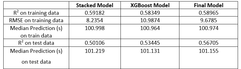Table 4: Final Model Performance Evaluation

There are number of important conclusions to be drawn from these metrics. The first is that the stacked model performs better on the training data but worse on the testing data than the XGBoost model. This suggests that the stacked model is overfitting the training data and the XGBoost model is better able to generalize to unseen data. In other words, the XGBoost model has a lower variance and higher bias than the stacked model.7 Therefore, averaging the two models means that the weaknesses of one are partly cancelled out by the strengths of the other. The final model does not perform as well on the training data as the stacked model, but it significantly outperforms both intermediate models on the testing data. The averaging of the two intermediate models is an acceptable solution to the problem because it leads to a model that is better equipped to handle novel vehicle configurations.

The final model is also more robust to changes in the input because it is an average of two different models. In order to determine the sensitivity of the final model, I manipulated the training inputs and observed the change in coefficient of determination on the testing and training set. I trained with and without the outlier using 140 principal components, and then altered the number of principal components and again recorded the coefficient of determination. The results are presented in Table 5.

Table 5: Sensitivity Testing Results

Across all training inputs, the R^2 score is very consistent. The model is therefore robust to variations in changes in the training data. If the results were highly dependent on the training data, it would indicate that the model is not robust enough for the task which is not the observed situation. Final results from the model can be trusted as indicated by the coefficient of determination score on the testing set. Although the model does not explain all of the variation in vehicle testing times, it explains more than half the variance and performs in the top 25% of the 3000 models submitted to the competition. The model would not be able to predict vehicle testing times for other companies because it depends on the precise features measured by Mercedes. However, given the problem objective of predicting Mercedes-Benz vehicle testing durations based on vehicle configuration, the model is useful.

Justification

The model outperforms the baseline on all relevant measures. The comparison between the baseline model and the final model are shown in Table 6.

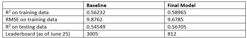Table 6: Final Model to BaselineComparison

The final model outperforms the baseline model by 4.86% in terms of coefficient of determination on the training set and by 3.95% in the same metric on the testing set. While these numbers may not seem large in absolute terms, they represent a significant improvement. This can be seen in the jump in leaderboard spots from the baseline to the final model. The baseline model placed near the bottom of the competition leaderboard at the 5th percentile, while the final model placed at the 75th percentile as of June 25. These results again show the diminishing returns of model optimization and the need for more quality and quantity of data. Even with a vastly more complex model, the overall performance did not vastly outperform the baseline and if Mercedes-Benz wants to obtain a better model, it will need to concentrate on obtaining more data. Nonetheless, a 4% improvement over the baseline could represent millions of dollars saved for a company that tests tens of thousands of cars on a yearly basis. In conclusion, the final model accomplishes the problem objective more successfully than the baseline and would improve the Mercedes-Benz vehicle testing process if implemented. As there is diminishing returns with respect to model optimization, additional improvements in the problem realm will only come from using more data.

V. Conclusion

Free-Form Visualization

In order to visually demonstrate the benefit of averaging models, I graphed the difference between the known target values and the predictions made by the stacked intermediate model, the XGBoost intermediate model, and the combined model. The result is shown in Figure 11.

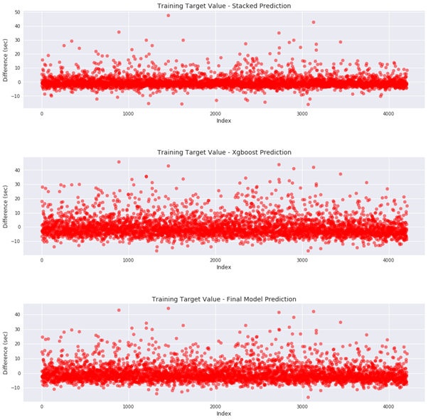Figure 11: Final Model Residuals on Training Data

This figure clearly illustrates the benefit of combining predictions from different models. The R^2 measure for the stacked model on the training data was much higher than that of the XGBoost model suggesting the stacked model overfits the training data. This can be seen by comparing the top graph of Figure 11 to the middle graph as the spread of differences between the known target values and the predicted target values is greater for the XGBoost model. The XGBoost model therefore has greater bias and less variance than the stacked model. Subsequently, the XGBoost model does not overfit the training data to the same degree as the stacked model, but it also might ignore some of the underlying relationships between the features and the target. While the stacked model does overfit to an extent, averaging in the prediction from the stacked model resulted in a better evaluation metric on the testing set. This indicates that the stacked model may be capturing a correlation on the training data that the XGBoost model did not incorporate while training. Overall, the final model is better able to handle new data because each weakness of the intermediate models is partially cancelled by averaging their predictions.

The second summary visualization also displays the benefits of combining the predictions from two different models. Figure 12 shows the individual models’ and the final model’s prediction on the training data (graphed against the assigned index).

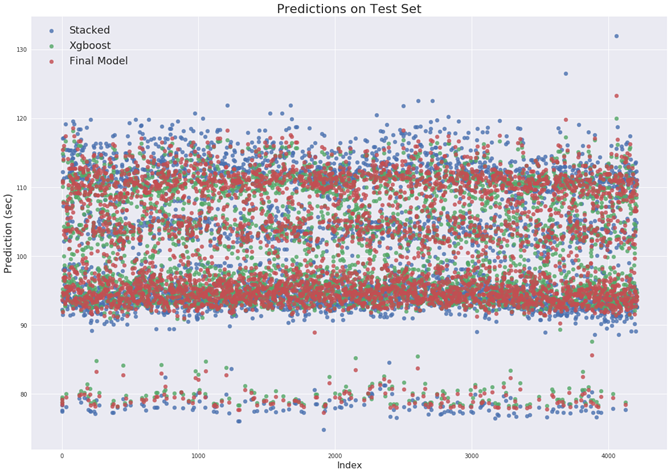Figure 12 Predictions on Test Data

The primary takeaway from this plot is that the stacked model has greater variance in its predictions on the new testing data in much the same way that it did on the training data. The spread of the stacked model predictions is much greater than that of the XGBoost model with the final model test set predictions nestled between those of the two intermediate models. Consequently, the final model is able to outperform both intermediate models. This visualization shows that combining models is beneficial and suggests that one possible method for further improvement would be to average in the predictions from additional different models. Each model will have its own biases and variance, but, much as averaging the predictions of a group of people is more accurate than that of a single individual, combining predictions from multiple machine learning model produces a higher-performing final model.

Reflection

This project represented the implementation of a typical machine learning workflow:

1. Data Exploration and Preparation

2. Data Preprocessing

3. Model Selection

4. Model Optimization

5. Model Testing and Evaluation

6. Reporting of Results

Completing a project based on a Kaggle competition had a number of advantages as well as several disadvantages. The biggest benefit is the availability of a clean dataset. Typically, machine learning projects will involve a substantial time investment procuring data and wrangling it into a usable format. That was not the case for this project because Mercedes-Benz made both the training and testing data available for download in a convenient CSV format. The first real step in this project was therefore data exploration. One of the major difficulties of this project was the anonymity of the data. No variable was given a physical representation (except for the target, the vehicle testing time) and therefore it was impossible to have an intuitive sense of the problem. This difficulty in interpreting the data influenced my decisions when it came time to preprocess the data. I decided to perform principal components analysis because it is an unsupervised technique that does not require an understanding of what each feature means. There were a number of options I could have explored, but for the final model, I decided that a PCA retaining 95% of the variance in the data was an acceptable procedure.

The second major difficulty of the project was deciding on the correct model. There are many more machine learning models than I would have thought possible at the onset of this project! I quickly realized that simple models such as a Support Vector Machine or a single Decision Tree were not going to be able to seriously compete. I therefore adjusted my approach and began researching ensemble methods, both in books, and in the Kaggle discussion forums. I read through many code examples that helped influence my final decision to go with an averaged model between two different models (with both intermediate novels incorporating ensemble methods). The final model I selected ended up being more complicated than I had initially thought, but it was justified in terms of the testing performance and the robustness offered by combining two different models. Optimizing the model was not overly difficult, but it did take a significant amount of research into the algorithms themselves and the meaning of various hyperparameters. I am grateful to the Scikit-learn community both for building such a user-friendly library and for providing the documentation needed to improve the models. Grid Search with cross validation proved to be an effective technique for bettering the algorithm scores and will always be a technique that I can rely upon when I do not intuitively know what the correct settings should be.

The testing of the model also proved to be a challenge because of the limited opportunities to try out models on the testing data. This was addressed mainly by using cross-validation numerous times on the training set, but those scores did not necessarily translate well to the testing set. This was the largest drawback from the Kaggle competition structure and I hope that Mercedes will release the targets for the testing set at the end of the competition to allow me (and the machine learning community) to learn how the models could have been better designed. Finally, the report itself has been a thoroughly useful experience. It helped to clarify my thoughts and encouraged me to understand my model in greater detail so I could communicate it to others. I know this is the most crucial aspect of any machine learning project because a model is only useful if its results can be applied. This almost always means involving other people and being able to explain how the model functions so others can use and improve upon the model. Moreover, I enjoying competing in the Kaggle competition because it gave me a chance to ask questions and interact with a community with a collective experience level far greater than any one individual can ever hope to acquire.

The final model is more complex than my expectations, but I believe it is appropriate for the problem. On future projects, I will approach the problem with the idea from the outset that a complex model might be required (although if the data is good enough, a simple model may be adequate) and I now have a better idea of what this type of framework looks like. I do not know if this exact model will generalize well to different problems, but the basic ideas behind it will. This project showed me the power of ensemble methods, particularly the XGBoost gradient boosting algorithm, and also the benefits of combining different models so that the weaknesses of one are cancelled by the strengths of the other. Overall, I thoroughly enjoyed this project and become much more involved with the community surrounding the competition than I had expected. I am eager to tackle more machine learning projects and it is encouraging to be in the midst of a rapidly-evolving field.

Improvements

The largest area for improvement is feature engineering. Most of the competitors at the top of the leaderboards used similar algorithms (some form of XGBoost stacked with other ensemble methods), and minor differences between scores were mostly the result of clever feature manipulation. [35] There were many approaches that were taken, including techniques such as Independent Components Analysis, Gaussian Random Project, Sparse Random Projection, and Truncated Singular Value Decomposition. I used only Principal Components Analysis because that was the technique with which I had the greatest familiarity. This is a poor excuse for not exploring other options, and that is my only regret with this project. I got too caught up with developing the model when I should have put greater emphasis on engineering the features. One common approach I saw among other competitors was adding the principal components to the existing features and then training on all of the features rather than reducing the number of features. This works because algorithms such as Random Forest and XGBoost learn which features are important during training by themselves, so it is not the job of the programmer to make that decision. My reduction of features was justified because I was still able to achieve a high coefficient of determination, but in the future, I may think about expanding the number of features rather than automatically trying to reduce them. Now that I know how to use Google Cloud, computing resources is not a significant impediment and I do not necessarily need to remove features in order to speed up training time. Moving forward, I will spend more time on feature engineering and less on perfecting the algorithm.

Another area that I would like to explore is deep learning, particularly with neural networks. [36] Although neural networks generally require many more training instances (as in millions rather than thousands), perhaps a properly designed neural network would be better able to learn the underlying relationships in the data. There were several competitors who tested out neural networks, but the leaders all used some combination of traditional ensemble methods. In the future, I might try a neural network for the practice and then implement one if I am using a much larger dataset in an industry setting.

In conclusion, I know that my model is not the best out there (as evidenced by my place on the leaderboard). I will continue to improve my model until the competition ends by redesigning the set of features and further adjusting the model hyperparameters. I am pleased with my performance and even more satisfied with the amount of knowledge that I was able to learn in throughout the process. In the future, I will be more prepared to spend a greater percentage of time on feature engineering and I know the level of model complexity that is required to perform well in these sorts of competitions. The Mercedes-Benz Greener Manufacturing Competition was difficult enough to challenge me but was also manageable for one getting started in the field. As an introduction to a complete machine learning project, I could not have picked a better problem to encourage me to continue moving forward in a field with great potential for improving our current systems.

VI. References

[1]. “Mercedes-Benz Greener Manufacturing Overview”, Kaggle.com, 2017. [Online]. Available: https://www.kaggle.com/c/mercedes-benz-greener-manufacturing. [Accessed: 20- Jun- 2017].

[2]. H. Schoner, S. Neads and N. Schretter, “Testing and Verification of Active Safety Systems with Coordinated Automated Driving”, 2017. [Online]. Available: https://pdfs.semanticscholar.org/ac7b/26a8df0609384ccf1593c7096665b2fd2e88.pdf

[3]. M. Tatar and R. Schaich, “Automated Test of the AMG Speedshift DCT Control Software”, 2010. [Online]. Available: https://www.qtronic.de/doc/TestWeaver_CTI_2010_paper.pdf

[4]. “Global Greenhouse Gas Emissions Data

US EPA”, US EPA, 2017. [Online]. Available: https://www.epa.gov/ghgemissions/global-greenhouse-gas-emissions-data. [Accessed: 20- Jun- 2017].

[5]. “About The Prize”, XPRIZE, 2017. [Online]. Available: http://www.xprize.org/about. [Accessed: 20- Jun- 2017].

[6]. L. Kay, “The effect of inducement prizes on innovation: evidence from the Ansari XPrize and the Northrop Grumman Lunar Lander Challenge”, R&D Management, vol. 41, no. 4, pp. 360–377, 2011. [Online]. Available: http://onlinelibrary.wiley.com/doi/10.1111/j.1467-9310.2011.00653.x/abstract

[7]. A. Géron, Hands-On machine learning with Scikit-learn and TensorFlow. O’Reilly, 2017.

[8]. D. Freedman and D. Freedman, Statistical Models: Theory and Practice, 2nd ed. Cambridge: Cambridge University Press, 2009.

[9]. “Finding R Squared / The Coefficient of Determination”, statisticshowto.com, 2017. [Online]. Available: http://www.statisticshowto.com/what-is-a-coefficient-of-determination/

[10]. “sklearn.metrics.r2_score — scikit-learn 0.18.1 documentation”, Scikit-learn.org, 2017. [Online]. Available: http://scikit-learn.org/stable/modules/generated/sklearn.metrics.r2_score.html. [Accessed: 20- Jun- 2017].

[11]. “Mercedes-Benz Greener Manufacturing Data”, Kaggle.com, 2017. [Online]. Available: https://www.kaggle.com/c/mercedes-benz-greener-manufacturing/data. [Accessed: 19- Jun- 2017].

[12]. D. Moore and G. McCabe, Introduction to the Practice of Statistics, W.H. Freeman, 2002.

[13]. “One-hot (dummy) encoding of categorical data in Excel”, Stackoverflow.com, Posted by user Chichi, 2015. [Online]. Available: https://stackoverflow.com/questions/34104422/one-hot-dummy-encoding-of-categorical-data-in-excel. [Accessed: 22- Jun- 2017].

[14]. “Skewed Distribution: Definition, Examples”, statisticshowto.com, 2017. [Online]. Available: http://www.statisticshowto.com/skewed-distribution/

[15]. L. Breiman, “Arcing the Edge”, University of California, Berkeley, CA, 1997. Available: https://www.stat.berkeley.edu/~breiman/arcing-the-edge.pdf

[16]. P. Geurts, D. Ernst and L. Wehenkel, “Extremely randomized trees”, Machine Learning, vol. 63, no. 1, pp. 3–42, 2006. Available: https://pdfs.semanticscholar.org/336a/165c17c9c56160d332b9f4a2b403fccbdbfb.pdf

[17]. D. Wolpert, “Stacked generalization”, Neural Networks, vol. 5, no. 2, pp. 241–259, 1992. Available: http://citeseerx.ist.psu.edu/viewdoc/download;jsessionid=BDDE4D399F09DA1275DAF5E444736A8F?doi=10.1.1.56.1533&rep=rep1&type=pdf

[18]. A. Charan, “What is a Decision Tree?”, Quora, 2016. [Online]. Available: https://www.quora.com/What-is-decision-tree. [Accessed: 27- Jun- 2017].

[19]. “sklearn.linear_model.LinearRegression — scikit-learn 0.18.1 documentation”, Scikit-learn.org, 2017. [Online]. Available: http://scikit-learn.org/stable/modules/generated/sklearn.linear_model.LinearRegression.html [Accessed: 20- Jun- 2017].

[20]. “Pearson Correlation: Definition and Easy Steps for Use”, Statistics How To, 2017. [Online]. Available: http://www.statisticshowto.com/what-is-the-pearson-correlation-coefficient/. [Accessed: 23- Jun- 2017].

[21]. “Mercedes-Benz Greener Manufacturing Leaderboard”, Kaggle.com, 2017. [Online]. Available: https://www.kaggle.com/c/mercedes-benz-greener-manufacturing/leaderboard. [Accessed: 20- Jun- 2017].

[22]. “Feature importances with forests of trees — scikit-learn 0.18.2 documentation”, Scikit-learn.org, 2017. [Online]. Available: http://scikit-learn.org/stable/auto_examples/ensemble/plot_forest_importances.html. [Accessed: 23- Jun- 2017].

[23]. L. Smith, A Tutorial on Principal Components Analysis. 2002. [Online]. Available: http://www.cs.otago.ac.nz/cosc453/student_tutorials/principal_components.pdf

[24]. “Choosing the right estimator — scikit-learn 0.18.2 documentation”, Scikit-learn.org, 2017. [Online]. Available: http://scikit-learn.org/stable/tutorial/machine_learning_map/index.html. [Accessed: 23- Jun- 2017].

[25]. “Mercedes-Benz Greener Manufacturing Discussion”, Kaggle.com, 2017. [Online]. Available: https://www.kaggle.com/c/mercedes-benz-greener-manufacturing/discussion. [Accessed: 20- Jun- 2017].

[26]. T. Dietterich, “Ensemble Methods in Machine Learning”, Multiple Classifier Systems, pp. 1–15, 2000. Available: https://link.springer.com/chapter/10.1007/3-540-45014-9_1

[27]. L. Breiman, “Bagging Predictors”, Machine Learning, vol. 24, no. 2, pp. 123–140, 1996. Available: https://link.springer.com/content/pdf/10.1023%2FA%3A1018054314350.pdf

[28]. L. Breiman, “Pasting Small Votes for Classification in Large Databases and On-Line”, Machine Learning, vol. 36, no. 12, pp. 85–103, 1999. Available: https://link.springer.com/content/pdf/10.1023%2FA%3A1007563306331.pdf

[29]. “XGBoost Documentation”, xgboost.com, [Online]. Available: http://xgboost.readthedocs.io/en/latest/model.html

[30]. D. Opitz and R. Maclin, “Popular Ensemble Methods: An Empirical Study”, Journal of Artificial Intelligence Research, 1999. Available: http://www.jair.org/media/614/live-614-1812-jair.pdf

[31]. “1.11. Ensemble methods — scikit-learn 0.18.1 documentation”, Scikit-learn.org, 2017. [Online]. Available: http://scikit-learn.org/stable/modules/ensemble.html. [Accessed: 20- Jun- 2017].

[32]. L. Buitinck, G. Louppe, M. Blondel, F. Pedregosa and A. Muller, “API Design for Machine Learning Software: Experiences from the Scikit-learn Project”, European Conference on Machine Learning and Principals and Practices of Knowledge Discovery in Databases, 2013. Available: https://arxiv.org/pdf/1309.0238.pdf

[33]. “Diminishing returns and Machine Learning: Increasing Gains

MIT EECS”, Eecs.mit.edu, 2016. [Online]. Available: https://www.eecs.mit.edu/node/6508. [Accessed: 27- Jun- 2017].

[34]. A. Halevy, P. Norvig and F. Pereira, “The Unreasonable Effectiveness of Data”, IEEE Intelligent Systems, vol. 24, no. 2, pp. 8–12, 2009. Available: http://clair.si.umich.edu/si767/papers/Week06/TextRepresentation/Halevy.pdf

[35]. “Winning Tips on Machine Learning Competitions by Kazanova, Current Kaggle #3 Tutorials & Notes

Machine Learning

HackerEarth”, HackerEarth, 2017. [Online]. Available: https://www.hackerearth.com/practice/machine-learning/advanced-techniques/winning-tips-machine-learning-competitions-kazanova-current-kaggle-3/tutorial/. [Accessed: 27- Jun- 2017].

[36]. Y. LeCun, Y. Bengio and G. Hinton, “Deep learning”, Nature, vol. 521, no. 7553, pp. 436–444, 2015. Available: http://pages.cs.wisc.edu/~dyer/cs540/handouts/deep-learning-nature2015.pdf

Appendix

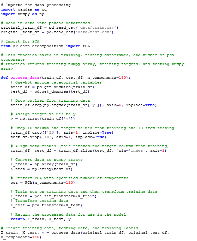
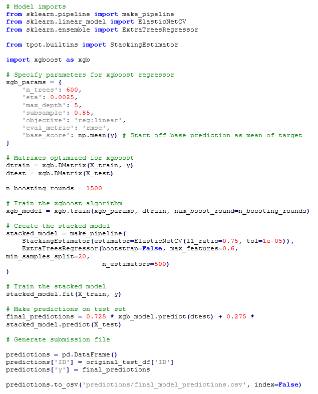
Final Model Code